Realistic Expectations While Monitoring with Networked Robotic Total Station Systems in Live Rail Environments.
Document
type: Technical Paper
Author:
J. Brzeski, Javier González Martí MSc MBA, J. Sánchez Barruetabena, ICE Publishing
Publication
Date: 31/08/2016
-
Read the full document
1. Introduction
Everything is in continuous movement, and the more precision with which we need to measure, the more difficult it is to get stable readings. The differences between two reading sessions can come from a number of different sources and events, from human aberrations during the transcription of readings, to minor accidental errors, changes in the atmospheric conditions, devices technical limitations, or even to real movements that are not directly linked to what we are intending to monitor (i.e. A change in the in-ground water layer, or even evolution on the tectonic rifts).
The more precise the movement we intend to measure the bigger the range of movement sources you get (Hope & Chuaqui, 2008). Although in big constructions we always assume that there is a limit to the project ZOI (zone of influence), this is not completely true, as they are under constant influence of several sources of movements and vibrations. Not only should the different monitoring techniques take this in account, the designers should also be aware of this in order to request and obtain quality readings from the different monitoring systems designed.
2. Monitoring concepts and specifications for Automatic Monitoring with Optical systems
Instrumentation and Monitoring (I&M) systems have evolved greatly in the last few decades and new applications of traditional techniques have also been developed. Without having a deep understanding of all the different I&M techniques it is challenging to decide which are the most suited to the problem at hand. As well as choosing the correct sensor one must also consider where to install them in order to get the required information and how to correlate the different information obtained. In the authors’ experience, these three questions of what, where and how are not often answered during the design stage, and are implemented once construction has started and there is a better understanding of the different constraints (real zone of influence, more accurate ground investigation, specific site visits from the different contractors, etc.). These concepts are further explored in (Cuevas, et al., 2012).
2.1 Definitions
It is necessary to define some of the terms that will be used during the article when reporting instrument performance. The following definitions are taken from (Dunnicliff J. , 1994).
- Resolution is the smallest division readable or measurable on the instrument. Interpolation by eye between divisions generally does not improve the resolution, as the estimation is subjective and operator dependent.
- Accuracy is the degree of correctness of a measurement, or the nearness of a measurement to the true quantity. The accuracy of a measurement depends on the accuracy of each component of the monitoring system. It is generally evaluated during instrument calibration, where a known value and the measurement value are compared.
Accuracy is expressed as ± ‘x’ units, meaning that the measurement is within ‘x’ units of the true value.
- Precision is the reproducibility and repeatability of measurement, or the nearness of each of a number of measurements to the arithmetic mean. Precision is also expressed as ± ‘x’ units, meaning that the measurement is within ‘x’ units of the mean measured value and is often assessed statically with a degree of confidence associated with the statistical distribution; a larger number of significant digits reflects a higher precision.
- Noise describes the random measurement variation caused by external factors. Excessive noise results in lack of precision and accuracy, and may conceal small real changes in the measured parameter.
Combinations of the above measurement uncertainties manifest themselves as measurement error, which is the deviation between the measured quality and the true value.
- Repeatability (this concept is not in Dunnicliff’s) is the variation in measurements taken by a single person or instrument on the same item and under the same conditions. It will describe how consistent an instrument is, taking into consideration all the possible errors affecting it, if any.
The following definitions are originally presented by Burland (Burland, 1995)[3]. The below are the factors usually related to structure damage control:
- Rotation or slope θ is the change in gradient of a line joining two reference points
- Relative deflection Δ is the displacement of a point relative to the line connecting two reference points on either side.
- Deflection ratio (sagging ratio or hogging ratio) is denoted by Δ/L where L is the distance between the two reference points defining Δ.
2.2 Automated Optical System though Robotic Total Stations
As automatic monitoring systems with Automatic/Robotic Total Stations can be quite controversial, every I&M specialist, or surveyor might approach this in a different way. At the present moment no standards have been set up, but all of them share some similarities, especially in the use of different components, such as prisms and RTS’s. The Robotic Total Station (RTS) automatic optical monitoring system consists of the following items:
- RTS: Robotic Total Station. Measuring device. Its location depends on the construction area; ideally it should be able to measure a minimal amount of references within an acceptable distance. As in most cases the size of the zone of influence exceeds the maximum distance of measurement so a networked solution is required.
- Monitoring targets: represent the monitoring points specified by the designer. These points are normally inside the zone of influence. The required frequency of measurement and visibility/distribution of these points will influence the amount of RTS’s to be installed.
- Reference targets: should be out of the zone of influence. Reference targets must be distributed in the maximum of directions (horizontally, vertically and in distance) around the station in order to provide a balanced reference system.
- Common targets: Are only used if the size of the area to be monitored requires the installation of several stations. These points allow the observations made from reference targets to be used by all RTS’s in the network.
- Hz: Is the angle that comes from the projection of the horizontal vector RTS-prism with the horizontal projection of the vector RTS-Hz0, where this Hz0 is a fixed point and the horizontal projection of the alienation with the RTS is the measurement of the horizontal angle. Otherwise related to the Azimuth
- V: Contained inside a vertical plane, this plane is perpendicular to a horizontal plane, and it is used to define the inclination of a line over the ground. Mostly related to the altitude, slope and zenithal angle.
- EDM: Electronic Distance Meter.
- ATR: Automatic Target Recognition.
RTS’s can work as standalone or group configurations depending on the requirements and constraints of the specific construction sites.
Once all the items are in place, the configuration of the system and processing of the data can differ from one company to another, but it will always follow surveying methodologies. Depending on how robust the data processing chain is, one will have more or less repeatable data. For the system related to this study, precision and repeatability have been more important than accuracy. For further understanding of these systems we advise referring to (McCormac, 1983)[12] and (Wilkins, Bastin, & Chrzanowski, 2003)[51].
In the author’s opinion a generic way of showing how one of these systems could work from the data collection phase, until the decision making phase is shown in Figure 1 below.
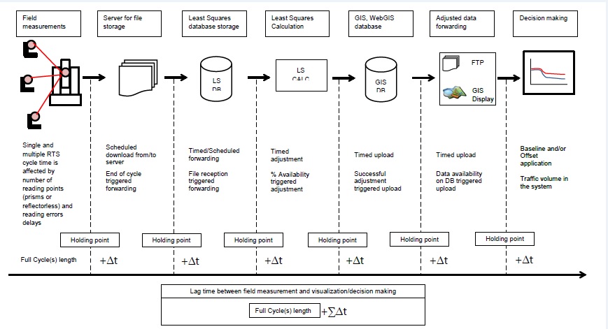
Figure 1 – Data collection to pressentation flowchart Although this generic flowchart (Figure 1) might vary from one contractor to another there is always a Data Collection Phase, a Data Processing Phase, and a Data Presentation Phase, and considerations should be made for each of them, in regards to how stable the data is going to be, and how is it going to be perceived by an end user. The main point of this article is to explore the first point and parts of the second one. Although the third could have a big weight on the final result as well it is considered out of the scope of this article and a discussion on this should be part of another study, or an extension of the present one.
2.3 Current contract specifications
In general, and in the authors’ opinion, the current Contract Specifications used in the industry, are not fit for purpose. This could be due to a lack of an industry standard on how to perform this kind of monitoring and also a lack of experience on the subject, as usually only the Monitoring Contractors have the specific technical knowledge of their systems.
An example of the clauses in contract documentation is given below:
“The quality of the accuracy and precision of the total stations shall be selected to achieve angular accuracy of 0.5 second of arc and distance measuring accuracy of ±1 mm + 1ppm”.
This demonstrates how the specifications tend to focus predominantly on the accuracy and precision of specific brands and/or models of instruments, stating that the supplier accuracies should be achieved, disregarding how the instruments have been set up, or if it’s an automated, semi-automated or manual set up, or any other possible factor that could affect the final accuracy and precision. The line is clearly referencing a technical specification that the RTS has to satisfy thus creating the perception that the final quality of the readings should satisfy them as well disregarding any possible local constraint such as weather, vibrations, natural movement, etc.
Other points often present in specifications are related to the frequency at which the prisms should be read, the maximum distance between RTS and prisms, the secure conditions of the machines, and the use of stable reference prisms outside the Zone of Influence (ZOI). Some specifications reference the need for correction of atmospheric effects and others also specify the requirement to monitor RTS bases in order to make sure that vibrations do not affect the system and or readings.
There are also the specifications of the 3D Geodetic prisms, where some of the specifications could be as bold as to state that “the quality and size of prisms shall be selected to achieve the accuracy of ± 1 mm”, indicating that the decisive factor on getting accurate data is the prism itself.
The specific sensors and instruments that will take the readings on the sensors are important to the final system accuracy, precision and over all repeatability, but as in manual monitoring, how the measures are taken and how the data is processed has a bigger impact on the final error, and as we will see how well the system has been designed prior to its installation. Not only should this be taken in account, but also that the variation on several factors (such as atmospheric conditions) will have an ongoing effect on readings and structures, having a toll in the overall stability of the data, which could be considered by some as inaccuracy of the system. This is where a robust post processing system can change things around and allow the system to have very repeatable data.
The specifications coming from the designer should cover only the information that the contractor will require in order to design a system which can achieve the desired monitoring results required in order to monitor the works.
2.4 Error evaluation and expectations
All the monitoring values, in terms of precision and accuracy, provided by the suppliers are on white lab conditions or on almost ideal conditions, which most of the time is not applicable to real site conditions, so we go from an expected “theoretical error” to a “real practical error” (Dunnicliff J. , 1994).
If we were to include all the possible errors that we could have in one specific system we should take into consideration:
- Error in the Electronic Distance Meter (EDM), depending on the supplier, ±1mm + 1ppm
- Angular error on the total station, about ±15 mgons on the newest models.
- Verticality error
- Collimation error
- Automatic Target Recognition (ATR) error
- Possible calibration errors
- Prisms constants (although not relevant in automatic systems, as nothing changes in the setup from one reading to the following one).
- Introduced errors while calculating the references through conventional surveying systems, and calculated through invers intersection and adjusted by least squares.
- Vibrations
- Atmospheric variations and their effect on the readings
- Obstructed/impaired lines of sight
- Human errors during the installation
As can be seen, it is difficult to provide a detailed final error for every sensor and/or for the overall system. This becomes more complicated if two or more RTS are linked in the same system as errors are accumulated from one to the other and subsequently adjusted through the entire system, making it difficult to understand unexpected behaviours.
Taking this into account it is more practical to provide the expected error (through error ellipsoids, or standard deviations) by performing a simulation once a preliminary (but achievable) design has been suggested. If the result is not satisfactory at this stage, the option of redesign is still available in order to try to improve the network.
In order to be able to perform a good simulation, estimate the system error and to be able to produce an overall design, the Monitoring Contractor should require/provide, as listed by (Gili Ripoll, 2008):
- Exact geometry of the area inside the relative or absolute grid used in the project.
- Exact positions of the RTS’s, angular position of the references and control points.
- 72h or more full day period (the best would be to arrive to a week) of readings to all the prisms on the system, if possible using Bessel. From here the contractor will have to define the quality of the readings over the period of time, distance and angular, and % of successful readings on every prism. Distance from the RTS to the prism should be provided as well, as higher variations are expected on higher distances.
- Final ATR accuracy for the model and brand used.
- Variation in the tilt of the RTS over the period of readings.
- Variation over the RTS position by performing resection with the reference prisms, and the variation of these prisms considering the RTS as a fix point. This should be provided in a graphical and numerical way (statistical analysis).
- Atmospheric conditions over the period of time. Thermic changes on highly isolated facades and possible correlations between points with high daily variations.
- History of ground movement episodes due to:
- Extreme ground temperature changes (i.e. Heave due to ground freeze)
- Water regime changes which could either be natural or induced. If induced it’s important to define the ZOI of this area.
- Potential big load changes in the area.
- Vibration map.
- Calibration or service plan in order to guarantee that the RTS are working to the supplier’s standards.
- Power oscillations.
The best way of being able to provide an estimate of the error is to analyse the raw data from RTS installed in different areas over the same period of time and at same time of the year (where we can assume similar atmospheric conditions). If the population is sufficiently large it should be possible to draw some meaningful conclusions from it and amend the design accordingly.*Note; after reviewing the data the Authors concluded that the set of data (error) was not normally distributed because the installation was already constrained by the technical specifications that did not permit the installation of monitoring prisms greater than100m from the RTS. Because of this constraint the Author were only able to allocate which were the main sources of error from analysing the Hz, V and Dcorr.
The same data should be analysed as well once it has been processed, as this will be able to show if the processing system improves the stability (repeatability) of the data, or not.
It would be worth mentioning the concept of “Real Time” in this section of errors and expectations. This term is misleading, and the source of many contractual claims and misinterpretations between the different parties. In the authors opinion, a Real Time Monitoring system should provide post processed data almost instantly, and these data should be revised/interpreted/assessed almost at the same time, which would be impossible in global projects (although maybe possible in small projects were the data feeds directly in to a local data base.
In the authors opinion the correct term should be Automatic Monitoring. The designer should specify how often the data should be made available and if the data is to be provided in raw or processed form as discussed in section 3.7.
3. Data Analysis
3.1 Real error or normal error
As explained in point 2.4, the best way of defining an error is by analysing enough data in order to define which the most common error is, although stating that there is just one error is quite a big statement, and probably misleading.
Since the RTS measure three parameters (Slope Distance, Horizontal Angle and Vertical Angle) we must analyse the effects of each variable on the standard deviation of the measured parameters in order to define this “normal error”. We have taken the data of 7 RTS over a period of one week, and studied the following parameters:
Slope distance variable
- Percentage of prisms observed vs slope distance (tD)
- Variation in vertical angle measured vs distance (vD)
- Variation in horizontal angle measures vs distance (hD)
- Variation in slope distance measured vs distance (dD)
Vertical angle variable
- Percentage of prisms observed vs vertical angle (tV)
- Variation in vertical angle measured vs Distance (vD)
- Variation in vertical angle measured vs vertical angle (vV)
Horizontal angle variable
- Percentage of prisms observed vs horizontal angle (tH)
- Variation in horizontal angle measured vs horizontal angle (hH)
- Variation in Slope distance measured vs horizontal angle (hD)
The study has been made with just one family of RTS, in such a way that the results should be comparable. This first family of RTS’s was installed in an open area, which will have a constrained vertical angle, since they are mostly installed on ground level masts, or on walls. The investigation should be completed with a second family with RTS installed in closed areas (mostly tunnels), understanding that they are mostly installed in the tunnels crowns, or at high level in lateral wall (although there are always exceptions), but because of the time constraints they were not included. As a note it has to be said that the data used in order to perform these analysis is coming exclusively from rail environments, which could introduce an error factor due to vibrations, less stable lines of sight, dust in suspension, etc.
All the data used has been extracted from areas that were considered to be stable at the time that the data was extracted.
Plots of the variables are given in figures 2-4 below with the Leica product specification details presented in table 1.
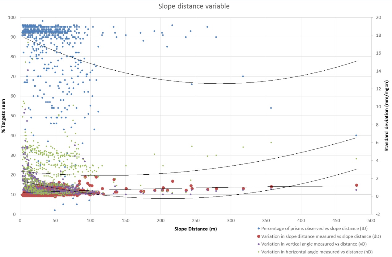
Figure 2 – Distribution of percentage of targets read and standard deviation of Distance, Horizontal angle and Vertical angle measured against distance from RTS. 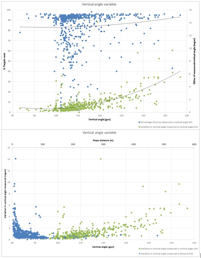
Figure 3 – Distribution of standard deviation in the vertical angle vs Distance and Vertical angle 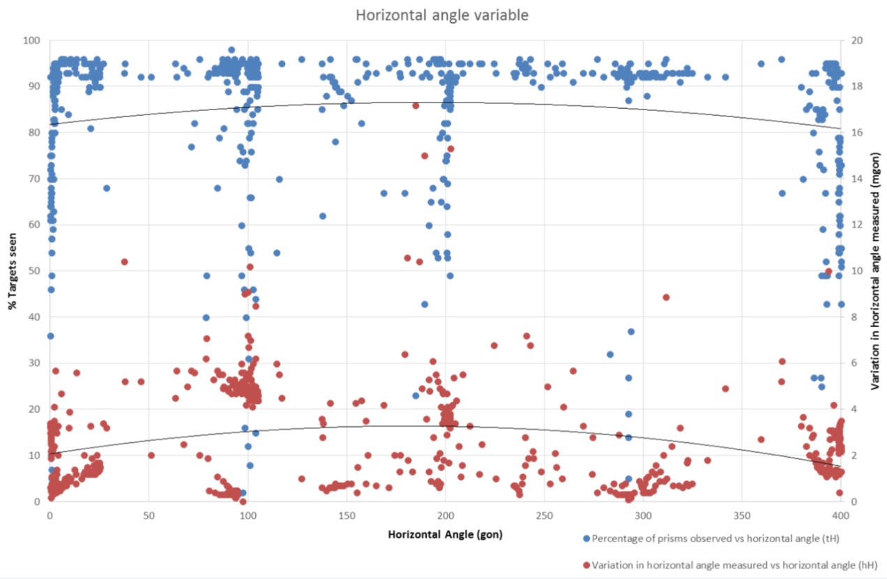
Figure 4 – Distribution of standard deviation in the horizontal angle measured vs the Horizontal angle 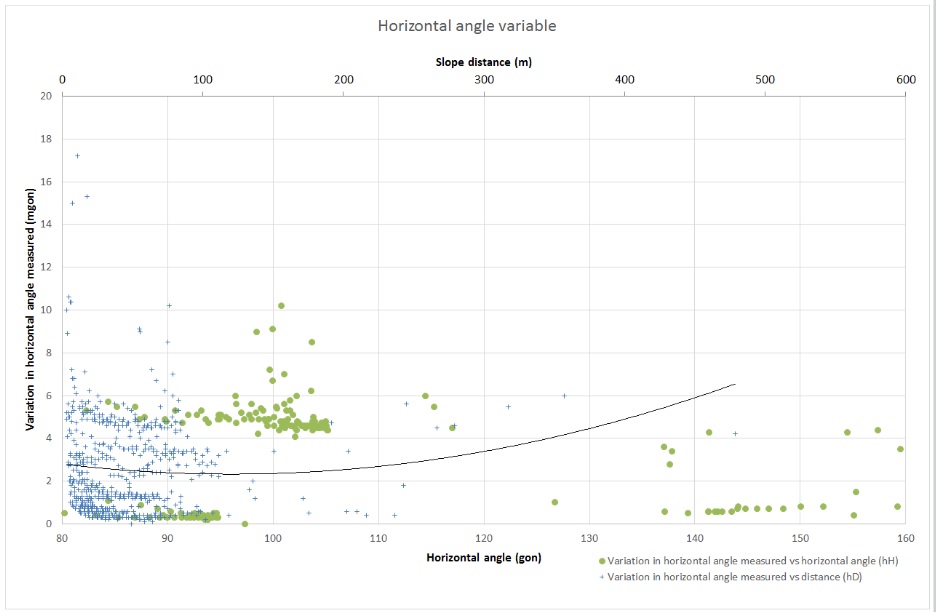
Figure 5 – Distribution of standard deviation of the horizontal angle vs distance 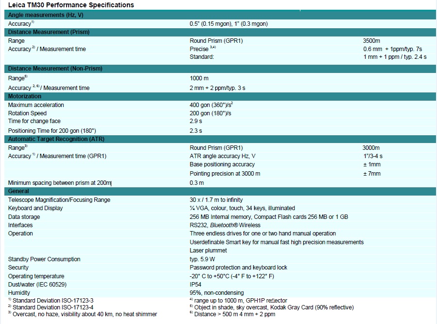
Table 1 – Leica TM30 Technical Specifications (Leica, 2009) From the graphs presented it is possible to derive the following information with regards to the errors observed.
Figure 2 demonstrates that the distance measurements are always under the accuracy given by the supplier, including on the furthermost prisms that are about 400m from the RTS. The source of error coming from this part of the reading is negligible.
Regarding the angle measurements, the accuracy is quite good (they provide a reference of the standard deviation of 0.15 mgon and 0.3 mgons), but the functionality that is used in order to automatically detect and read the prisms, the Automatic Target recognition (ATR), has a poorer performance, and will introduce more error in to the data.
The angular standard deviations presented in Figure 2 suggest an increase in the standard deviation of readings from the prisms that are closer to the RTS, up to about 30-35 m, for both Horizontal and Vertical angle, which afterwards becomes constant albeit it with a high degree of scatter, especially in the horizontal angle. As well that the error coming from the distanciometer remains well below the millimetre. Both of these conclusions are aligned with the supplier’s information on their equipment (table 1).
What is not so obvious, or clear from the suppliers information is that in close distances, from 0 to 35 meters, the ATR does not perform well, and can arrive even to levels of 7-8 mgons, in either the vertical or horizontal angles.
Figure 3 shows a positive correlation between the vertical angle and variation in the reading of the same. This is most likely a function of the ATR also as a steeper vertical angle indicates a closer target.
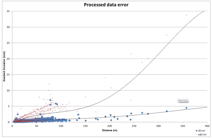
Figure 6 – Final process error vs angle and distance Figure 6 shows the error distribution taking in consideration the following formula:
Delta angle[gon]*pi*distance[m]/200 = error [m]
There is a last consideration to be made which has been as well consistent across all the samples studied. Prisms with low percentages of readings provide high deviations in the Vertical and Horizontal angles, and potentially even in the distance.
Many of the Monitoring Contractors and/or Designers tend to constrain the distances between RTS and Prisms, stating that this is necessary in order to guarantee the quality/precision of the readings. This constraint has been found to be misleading although it is constant with the plot presented in Figure 6. It has to be taken in consideration the availability of the refs in order to be able to have a consistent and stable network configuration. This can be seen in the process data results of this specific family of RTS’s in point 3.2. The error up to 200 m is below 2 mm, so 200 m should be an acceptable distance. After 200 m the error grows faster. Table 2 shows the distribution of the prisms in this study, it can be seen that this should be optimised so that the number of prisms is increased in the optimum range of 35 to 200m.
Slope Distance % of prisms Number of prisms 0-50 65.56% 316 50-100 29.46% 142 100-150 3.53% 17 150-200 0.41% 2 200-250 1.04% 5 Table 2 – Distance vs % of installed prisms
Another factor to consider is the number of prisms per RTS. It is generally accepted that the instruments should read all its monitoring targets in a cycle of no longer than 1 hour. This routinely equates to around 120 prisms. Table 3 shows correlations of RTS vs Prisms installed and maintained for Crossrail over an extended period of time. As it can be seen in the last column, the average of prisms per RTS was 83 prisms regardless of the number of RTS.
Date RTS [NB] prisms [NB] Prisms per RTS 07/04/2014 204 16780 82 14/04/2014 200 16478 76 20/04/2014 185 15096 89 11/06/2014 184 15045 87 07/07/2014 184 14976 90 04/08/2014 184 15127 83 01/09/2014 184 15200 79 06/10/2014 152 12682 79 27/10/2014 151 12604 79 24/11/2014 159 13031 83 01/12/2014 156 12826 82 08/01/2015 151 12341 84 19/01/2015 145 11923 82 24/03/2015 144 11958 80 31/03/2015 134 11054 82 28/04/2015 133 11022 81 26/05/2015 130 10639 83 22/06/2015 113 8932 86 06/07/2015 104 8614 82 14/07/2015 98 8024 83 16/08/2015 98 8024 83 Table 3 – Correlation between numbers of prisms read per RTS
The conclusion from this analysis is flagging once more the importance of a previous design and analysis, which in this case would have raised that:
- RTS’s should not read prisms closer than 35 m.
- There is not a clear limitation in distance, so the limitation will be either the amount of prisms to be read, or the shape of the area to monitor. This should mean a saving for the client by installing less RTS’s (not only in the device and installation, but as well all the paper work and maintenance behind them).
- Pre-design and pre-analysis is pivotal in order to understand the repeatability / accuracy constraints.
3.2 Error compensations though Network configurations
The same analysis described in section 3.1 above is also carried out on the processed data to assess the impact the network adjustment has on the raw data. In this case there are more considerations to be made, as for instance that the networks will have RTS’s in exterior areas, and in interior ones, and that some of the networks could be more stable than others (for the reasons already explained on point 2.4).
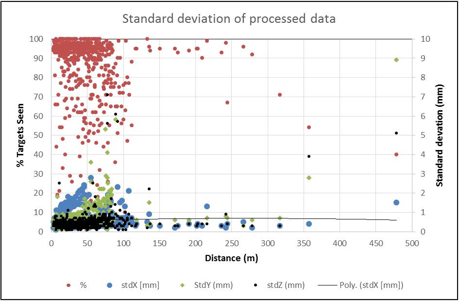
Figure 7 – Standard deviation of the process data through the network configuration As can be seen, once the data has gone through the network configuration / calculation process, and because of the different weight distribution that different references and common prisms will have, the process data does not present the same kind of errors than the raw data. As can be seen in Figure 7, the Z values are mostly bellow 1 mm, and the X and Y are slightly bigger (up to 2 mm), but they are mostly depending on the Network configuration, and the % of readings, not on the quality of the data itself.
3.3 Influence of Network adjustments on RTS readings
The Least squares-based software adjusts the measurements taken (Hz, V, Dist) based on an initial configuration that has proven stable and robust and a set of tolerance values that guarantee a degree of flexibility. The new or latest measurements are compared against this geometry and the discrepancies between the actual and the ideal networks are represented in the form of residual tables, for example. In order to minimize these residuals the measurements go through and iterative process that will stop in the event that the geometry achieved falls within the network’s tolerance or terminate in the event that after a number of iterations convergence is not achieved.
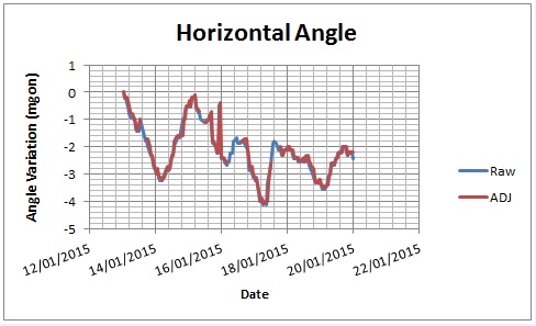
Figure 8 – Single prism raw vs adjusted horizontal angle readings 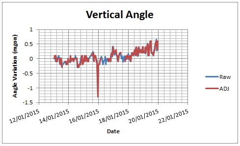
Figure 9 – Single prism raw vs adjusted vertical angle readings 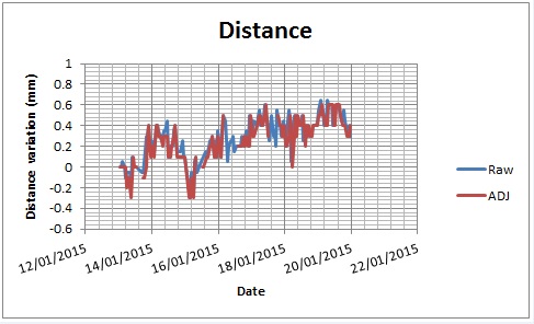
Figure 10 – Single prism raw vs adjusted distance readings Figures 8 to 10 above show a comparison between the angular and distance measurements before and after the adjustment on a prism over time. It can be appreciated that the adjustments match spikes and carry on with the trends if by some reason the least squares (LS) process has stopped working. It is quite noticeable that the distance values for this specific prism require a higher amount of adjustment as the original readings have less overlapping in some areas.
The opinion of the authors is that the usual philosophy in LS configurations should be aimed to adjust the original readings as least as possible in order to achieve an acceptable network geometry. Adjusted readings that minimize the accumulated error whilst remaining true to the original readings allow the addition of QA controls and alerts in case the network might be compromised by a temporary or permanent shortage of network elements (common points or references).
Although requiring a higher level of surveillance, these practices prevent network decay through loss of prisms or links between network elements as a result of non-effective maintenance or third party disturbance.
3.4 Natural fluctuations on standalone RTS’s
As raised in point 2.4, variations on the atmospheric conditions will have an impact on the data. These conditions will affect the structures being monitored and also the readings taken by the monitoring devices. This is what many monitoring contractors will call as the individual “Thermic Structural Signature”.
It is true that all structures tend to have their own natural behaviour, which will mostly depend on factors such as isolation, construction material, if it’s inhabited or not, internal structure and ventilation systems, height, wind speed, etc., It is also known that many tall buildings can have a big sway (i.e. The Sears Tower of 442m, sways up to 300 mm with strong winds). In general it is accepted in the industry to have this kind of behaviour, although it is not desirable, and many times leads to misinterpretations, analysis errors, and overall dissatisfaction from the client, although most of the monitoring contractors will tend to explain that there is nothing it can be done about it.
Whether the authors accept that these movements do exist, and that a change in the temperature (or other factors), season, or time of day, will affect the structures, what is provided by the monitoring contractors is not really only that variation, but a sum of added factors.
Because of the way the systems are configured, for the most part (by using references outside the ZOI) in order to calculate the RTS position each cycle (process session), every time that the adjustment is done the system defines a new reference axis from which the calculations will be done. Depending on how homogeneous/heterogeneous the system is the more stable the readings will be.
The following seeks to illustrate this effect in the case of a single RTS installed on a high building measuring references at the same height of the RTS and monitoring prisms on a similar height, and two other lower levels (as per Figure 11).
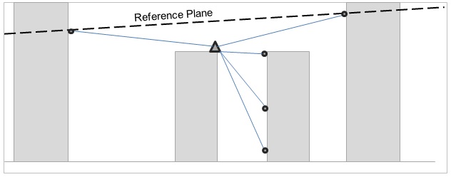
Figure 11 – Draft of an RTS installation monitoring prisms at different height. Most likely the fluctuation of the structures with similar heights should be the same (providing that they are made with similar materials, which tend to happen on one specific small area (a radius of about 100m). The reference plane define by the refs will be approximately at the same height of the highest control prisms, which in principle should be the ones detecting more movement because of the inherent behaviour of structures to thermal change and other environmental effects.
The reality is that because the behaviour of the reference axis calculated though the references has a similar daily oscillation that the high level prisms installed at its same height, and so would be the calculated RTS position (and most likely physical as well), the distance between them is more stable than the distance vs the other prisms. The effect seen in the plots is that the thermic oscillation is most evident on the low level prisms, and middle ones, and very mild or not existent in the high level ones.
The final point is that the “Thermic Structural Signature”, is always a combination of the noise introduced by the fluctuation of the reference axis, and the real signature of the structure. In the authors’ opinion and until the monitoring contractors processing systems (or post processing systems) has improved, or the industry standards of a higher technical quality, this should be considered as “noise”, and the data should be able to be adjusted through a polynomial regression that is able to provide a best fit.
The way of minimising this behaviour is to manage to get a very heterogeneous reference prism distribution, in such a way that the reference axis will be compensated, unfortunately this is often very difficult to achieve in reality, due to the specific constraints in the areas that require this type of monitoring.
3.5 Natural fluctuations of network configurations
Now that we have defined the difficulty of getting clean data from these monitoring systems when they are working as individual RTS, the introduction to network systems is easier, as the same errors (calculation process) apply, plus one addition, the common prisms and the network configuration itself, that will constrain how the errors are distributed along the length of the system.
On surface areas, where the RTS are either fixed to building facades, on masts, or on the top of buildings, obtaining a good special distribution is possible, but on rail environments this is far more challenging, as not only are you constrained to a track geometry (which by nature is quite linear), but also tunnels, H&S limitations, overlapping lines of sight, intermittent but constant obstruction of the lines of sight, vibrations, grease and dust that will cover the prisms and RTS lenses, aggressive dust in the RTS servos, etc. All these factors will impair the performance of the system if mitigations are not put in place (such as a constant maintenance of the system).
Because of all these variables present in rail environments, providing noise free readings is difficult, and the possibility of introducing a bias is quite possible if a constant control is not in place. QA and KPI’s are critical to ensure the good performance of the system.
The principle behind a long network installed in a tunnel is similar to a string in a guitar; both ends of the string remain fixed and tight by an element (references) and allow movement in the middle part of the mast. Common targets are (normally) used to keep the network as tight as possible in the middle, without the weight of the reference points.
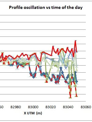
The following figure depicts the effect of a network edge too constrained in one edge and how the lack of fixed points along the network allows a certain degree of oscillation. The example illustrates less than 100m of rail profile and the values were obtained through a one week average calculated for each hour of the day. To simplify the representation the values have been represented every 4 hours.
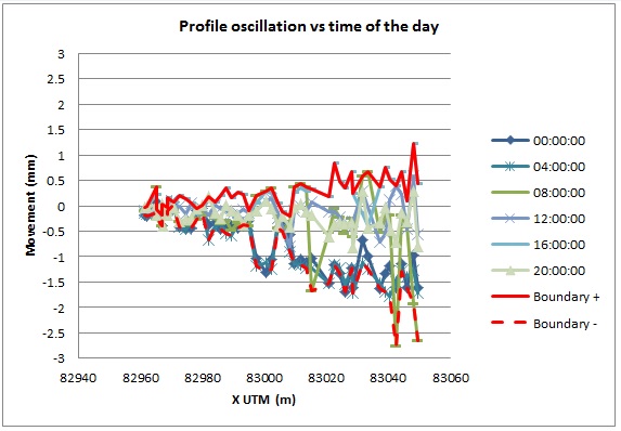
Figure 12 – Example of the edge of an RTS Network illustrating the reference influence and daily oscillation on a rail profile The effect of the references fades out as the trends move West the network is less constrained and reflects the combination of noise and temperature changes in the area.
A similar study has been made over a longer profile (>250m) to reflect its evolution in a four-day period. In this case the plots are composed of a daily average, and the maximum and minimum values reached on that day to illustrate the difference between the highest and lowest reading of a prism profile vs the behaviour of the daily average.
The oscillation that the network experiences over such a short period of time whilst keeping the daily average close to the reference level 0 shows that a number of factors are affecting the daily readings in this area and producing a level of noise/oscillation that can be removed by summarising the daily readings using methods such as a median or an average that will produce much more understandable profiles or trends.
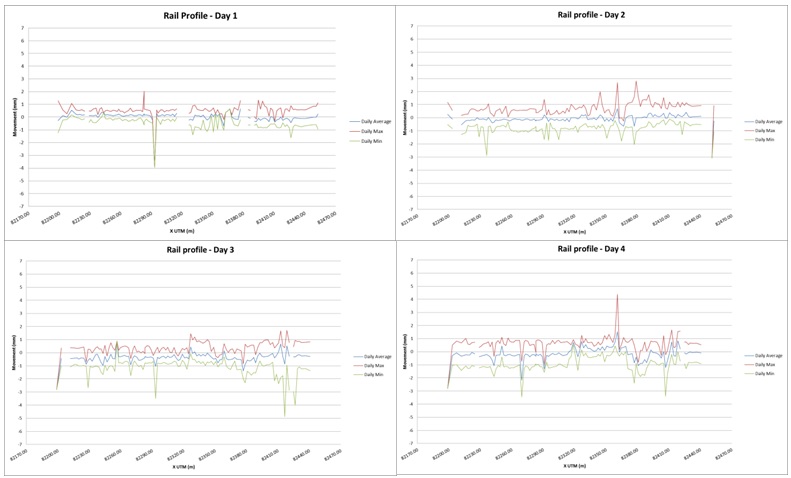
Figure 13 – 4-day evolution of a profile (Note: Spikes bigger than +/-5 mm have been removed) 3.6 Post processing
Many I&M contractors and/or Principal Contractors are of the opinion that their only obligation is to provide raw and pure data adjustments (with one or other software), and any further work from there deviates from their obligation, as it can be considered as interpretation of the data. Others hide behind strong processing systems in order to state that their data is better than others, when what is really better is the post processing of it, but without explaining to the client the different processes that this data improvement involves.
In the authors opinion post processing of the data is vital, and is be something that the contractor should (following the designers specifications) do in order to mitigate the many sources of errors explained in point 2.4, which will produce “spiky” or erroneous data. But as well in the authors consideration, the Monitoring Contractor should clearly explain all the steps of their process and post-processing system to the client, in order for the client to be able to decide what is the best set up in each case in order to get the best and most meaningful data in their project depending on their specific constraints, which might change in the time, as can change the initial post-processing set up.
The concept of repeatability comes in to place when processing and/or post-processing of the data is done.
If these constraints are not well defined, or they are not made aware to the client, not only could it mislead the client’s engineers, but it could be considered that the Monitoring Contractor is deliberately misrepresenting the actual site conditions.
4. Designing and defining monitoring systems. QA & KPI’s
As explained so far, monitoring with RTSs has its issues, this is why the authors, based on their experience have tried to provide a matrix (Table 4) suggesting the type of monitoring to be used depending on the type of project, of course it is quite difficult to tick all the boxes that will be found on every other project, so it has to be used taking in consideration the individual characteristics of the project.
Application Manual Monitoring Automatic Monitoring with 3D prisms Tiltmeters Chains Photogrammetry Water Settlement Cells systems INSAR Precise Levelling 3D Monitoring Z X Y Z X Y Z Z Relative Displacements Z Z TBM Tunnels. Urban Areas Low Risk + – – – – – – – – – + TBM Tunnels. Urban Areas High Risk + ± ± ± + + + – – + + TBM Tunnels. Rail Environment Low Risk + ± ± ± ± ± ± – – – – TBM Tunnels. Rail Environment High Risk + ± ± ± + + + + + – – SCL Tunnels Urban Areas + ± ± ± + + + – – + – SCL Tunnels Rail Environment + ± ± ± + + + – – – – Shafts / Boxes + ± ± ± ± ± ± – – – – De Watering + ± ± ± ± ± ± – – – + Compensation grouting ± ± ± ± + + + ± – + – Table 4 – Project type vs monitoring system ( + Likely to be used, ± Possible to be used, – Unlikely to be used)
The Authors have defined a risk matrix indicating which party holds the risk with regards to the known causes of errors in RTS systems (Table 5).
Serious High Level Low Level Known/Accepted Supplier Instrument not performing correctly. Instrument not well calibrated. Systematic error due to instrument performance Designer Erroneous or misleading specifications. Erroneous ZOI. Erroneous delimitation of the trigger levels. Error in the definitions of the requirements from the monitoring system Monitoring Contractor Network configuration and system in general, not well maintained QA & KPI’s not in place in order to check RTS’s calibration before and while they are in use. Error &/or noise due to the specifics of the system. Error definition after simulation. Errors in the processing system. Network evaluation & analysis not well done or applied. Table 5 – Risk matrix for know sources of errors in RTS networks
4.1 Technical Limitations
There are other considerations to be made, that are not linked to the systems technical specifications (point 2.3), the system’s inherent constraints (2.4), the real error (point 3.1), the Monitoring Contractor system robustness (point 3.2 & 3.7), or the natural fluctuation of the systems / Networks (point 3.6).
In this aspect we would like to enumerate some salient points:
- Experience and robustness of the Monitoring Contractor Design and Simulation Systems.
- Technical flexibility in order to suit the different constraints. I.e. being able to use different communication systems like GSM, Wi-Fi, direct lines, etc… depending on the site constraints.
- Robust data acquisition software.
- Remote access to the acquisition software and custom made options. I.e. in order to be able to operate the RTS’s remotely without having to be on site for it.
- Robustness of the entire process and internal QA checks.
- Automatic system reboot
- Internal cyclic adjustments
- Automatic triggering systems
- Quality of the least squares adjustment formula, and how much can be tailored in order to take more factors in consideration.
- Visualisation system
All these points will have an impact on how successful the presentation of the data is.
4.2 QA & KPI’s
The information should be provided in a timely manner, depending on the criticality of the project, but for this specific case of monitoring live track environments, we recommend at the very least a daily check is carried out, more likely twice per day.
Having triggers and daily and weekly performance checks is critical in order to be able to maintain optimal system condition, and to be able to identify possible sources of error.
The factors that the Authors consider that are critical are:
- From the RTS.
a. When was the last data set received (in minutes).
b. Total number of prisms read one time (at least) since the last report vs total of prisms read by the RTS.
c. Maximum % of prisms read since the last report.
d. RTS inclination (level).
e. Battery power. - From the processing system.
a. When was the last data set processed.
b. Deviation in Horizontal Angle
c. Residuals from references.
d. KPI for general performance of the group (sigma).
e. Performance of each RTS, if below 95%, as a time plot.
f. No. of not read prisms per network and per amount of days without a reading.
g. % of prisms read as a time plot. - From post processing the readings
a. Standard Deviations for X, Y and Z over a day – week – period.
b. Tilt of RTS over the same periods.
c. Correlation between events and % (maintenance, RTS failures, comms failures, etc.)
Decisions should be made on these reports and the priority / criticality of the works being monitored by the system.
4.3 Maintenance
A daily maintenance of the systems, software and hardware (including prisms), is critical in order to be able to provide satisfactory prism reading percentage.
For this is necessary to plan ahead, and be observant on the patterns that can develop overtime, once again (as explain in Point 9 as a short case study), the design is critical
Simple precautions like orienting the prisms against the train advances could have a big budget impact by lowering the cleaning activity on the lenses as demonstrated in the case study presented in Section 9.
5. Final specifications and considerations for Networked system with RTS.
The following considerations must be taken into account when writing specifications and when designing systems such as this.
- The assessment of ground movement will be provided to the Monitoring Contractor. The assessment will include a delimitation of the project ZOI, and clearly state which component the designer will require information on (settlement (Z), movements along the X and Y axis).
- A clear definition on what is to be understand by X, Y and Z (i.e. If they are absolute to a specific grid, and their relation to it, or relative to each surveyed structure)
- The contractor will be provided with any other possible relevant information, such as stratigraphy, phreatic levels and regimens, type of foundations on the buildings around the project (if available), construction phases and description, etc…
- The designer will provide the expected degree of repeatability between two sets of data, and the level of certainty that is required for that data.
- The designer will define the needed frequency between data sets, and state the time delay between the time that the data is collected (raw data), and when it has to be available after any post processing (processed data), related to the decision making phase (Fig. 1)
- The contractor will have to suggest a design, system of work, data collection process, processing system, post-processing system and all the QA and KPI’s that should be in place on every step in order to be able to satisfy the designer’s requirements. In case that these requirements are not achievable, the contractor has to clearly state this, and provide what could be achievable with their systems, and what it implies for each of the previous steps. In order to provide this information a design and a simulation are pivotal.
- It should be an iterative design, as imperfections will arise
- The Contractor should ensure that sufficient levels of redundancy exist in the design of all parts of the system.
- The contractor has the obligation of providing enough detail regarding their different processes, systems of work, processing, and post-processing system and options in order for the client to have confidence and understanding of the system prior to installation.
- The contractor must provide a report giving the limitations of their system (i.e. How far/close a prism has to be in order to suit the contract requirements), taking in consideration the system as individual RTS’s and sensors, and the system as a network. They need to be able to suggest possible improvements that could be made if the contract requirements are not satisfied with the accepted budget, and the cost implications.
- All the information should be backed up with diagrams and simulations.
- The equipment to be used has to be agreed with the client, and has to be up to the best industry standards in order to be durable over the full period of the contracted works. All kind of considerations should be made in order to suit the system and components to the site specific conditions.
- Maintenance of the equipment and the system has to be considered until the decommissioning phase.
- Manufacturers guidelines with regards to maintenance of equipment should be adhered to.
These points could be used as a very general guideline, but each contract should have their own contract specific considerations/requirements.
6. Conclusions
The main conclusion to be drawn from this study is that although monitoring through RTSs has been done for over 15-20 years and is the most utilised form of monitoring, there is very little knowledge about them. This is due in part to the novelty of the systems, the monitoring contractors retaining their system setup, and a lack of industry standards.
If there was a well-defined and accepted technical specification standard, it could lead to a better system definition, which would force contractors to increase their own standards, and assist the client technical teams in providing better contract designs and definitions. All these improvements, would not only lead to fewer contractual disagreements, but would also save budget thanks to better and more optimised designs by using fewer RTS to monitor more prisms in the optimal prism range of 35 to 200m as shown in section 3.1.
High levels of performance have been achieved by a continual review process in order to fine tune previously installed networks, determining appropriate Key Performance Indicators for quality and regular maintenance of monitoring and system targets.
It’s imperative that industry standards area created and accepted, and large scale projects, where large amounts of instruments are installed are the ones that push these standards.
8. Bibliography
Burland, J. B. (1995). Assessment of risk of damage to buildings due to tunnelling and excavations. Proceedings, 1st International Conference for Earthquakes and Geotechnical Engineering.
Cuevas, M., Zarzosa, L., de Las Nieves, M., Andres, N., Amparo, M., Ripol, G., et al. (2012). Ensayo a escala real de varias técnicas geomáticas de monitorización de movimientos de edificios. Congreso Iberoamericano de Geomática y Ciencias de la Tierra. Madrid: Ilustre Colegio Oficial de Ingenieros Técnicos en Topografía de España.
Dunnicliff, J. (1994). Geotechnical instrumentation for monitoring field performance. Wiley.
Gili Ripoll, J. A. (2008). Informe asesoria sobre sistemas de moniotorizacion de movimientos de superficie durante obras subterraneas de nuevas lineas de FFC en zonas urbanas. Universitat Politecnica de Catalunya.
Hope, C., & Chuaqui, M. (2008). Precision Monitoring of Shoring and Structures. Field Measurements in Geomechanics (FMGM) Symposium Proceedings. Boston.
Leica. (2009). TM30 Datasheet.
McCormac, J. C. (1983). Surveying Fundamentals. Prentice Hall PTR.
Wilkins, R., Bastin, G., & Chrzanowski, A. (2003). Alert: A fully automated real time monitoring system. Proceedings, 11th FIG Symposium on Deformation Measurements. Santorini.
9. Case Study
Purpose
The purpose of this study is to evaluate the impact on track and structure prisms of a live track environment with close to 24/7 train circulation over a 4-month period between January and April 2015
Scope
The area chosen covers the southern end of Farringdon Thameslink NR station from the Cowcross St Bridge to the southern end of the NR platform
Site description
The section of the asset to be monitored is the extension of the Thameslink platform, built to allow the use of 12 car trains which was completed in time for the 2012 Olympic Games. The section is approximately 90m long.
The monitoring equipment installed in this asset to monitor CRL activities comprises 3 total stations and a total of 241 monitoring prisms, 121 installed on the tracks and 120 on the surrounding structures (platform nosing, columns, etc…).
Site conditions
The continuous use of the line places an extra amount of stress into this optical monitoring installation whilst also makes its maintenance difficult. Brake dust from the trains is the principal element that interferes with the track prisms alongside with random knocks caused by third parties. The structure prisms are less exposed to this type of wear and usually require less maintenance.
The line is only closed to rolling traffic one night per week and many different parties can access it to perform different tasks, this makes unscheduled access difficult to accomplish. Late access and early site leaving situations happen quite often limiting the maintenance time which is critical when Total station(s) and prism maintenance has to take place.
Dataset
The readings used span from the 9th of January 2015 to the 9th of June 2015.
The readings used belong to total stations No’s 7, 8 & 9. There is an additional one (No 10) that covers the cut and cover tunnel that malfunctioned twice during the study period, in one of the occasions for almost two weeks, to differentiate those episodes from the maintenance related system degradation the readings of that Total station were removed from the dataset.
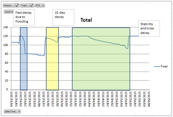
Maintenance rounds over the study period
Four Prism clean maintenance rounds took place over the abovementioned period on the following dates: 17/01, 14/02, 28/02, 17/05 with different levels of prism recovery as can be seen in the following figure.
Exceptional conditions
On the 23rd of January 2015 a broken main poured around 50.000 litres of water in the tunnel between King’s Cross and Farringdon Stations, that meant that the train service was put on hold between those stations but also that the prisms installed in the down line (trains towards Brighton) were covered in dirt and ceased to be usable reflectors until the next maintenance round on the 14th of February.
Prism trends analysis
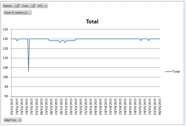
Structure
Prisms placed in the station’s structure have proven to be more resilient as tend to be high enough to be free of train circulation spills, dust or similar products emissions. This can be seen on the following figure, which exemplifies how the amount of prisms read remains quite constant
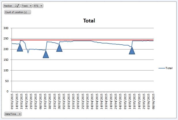
Track
Track prisms are more vulnerable any products spilled or carried by moving trains, as well as easy to knock by human or mechanical means as they move along the tracks during engineering hours. During the study period there are three periods that reflect how the amount of prisms read diminishes in time as they progressively lost their optic properties.
There are three periods that exemplify this phenomenon:
- 18/01/215 to 24/01/2015. Prisms lost because of the flooding in Thameslink line. The prisms located in the down track were affected by the moving and stopping trains as were facing opposite to the train’s moving direction, the trend builds up quickly and then stops, as no more prisms accumulated enough dirty after this episode. The trend slowly builds up again from the 4th of February until the maintenance round on the 14th but is very mild in comparison.
- 15/02/2015 to 28/02/2015 trend in between maintenance rounds shows which is much less steep than the previous
- 28/02/2015 to 16/05/2015 this period can be separated into two trends. The first one is a stable period that lasts until the 3rd of April approximately in which there is little variation in the amount of track prisms read. The second period starts at that point and displays a trend similar to period 2 and goes on until mid-May. This period is useful as allows the mapping of the gradual system deterioration.
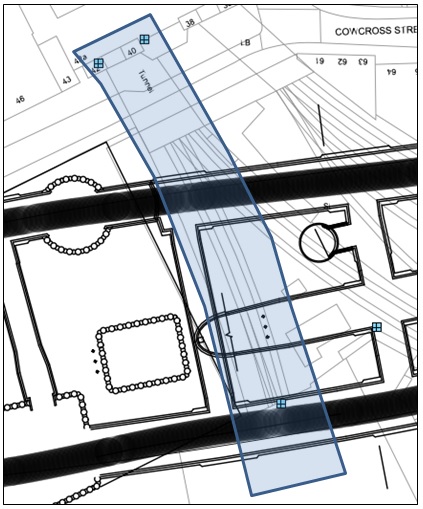
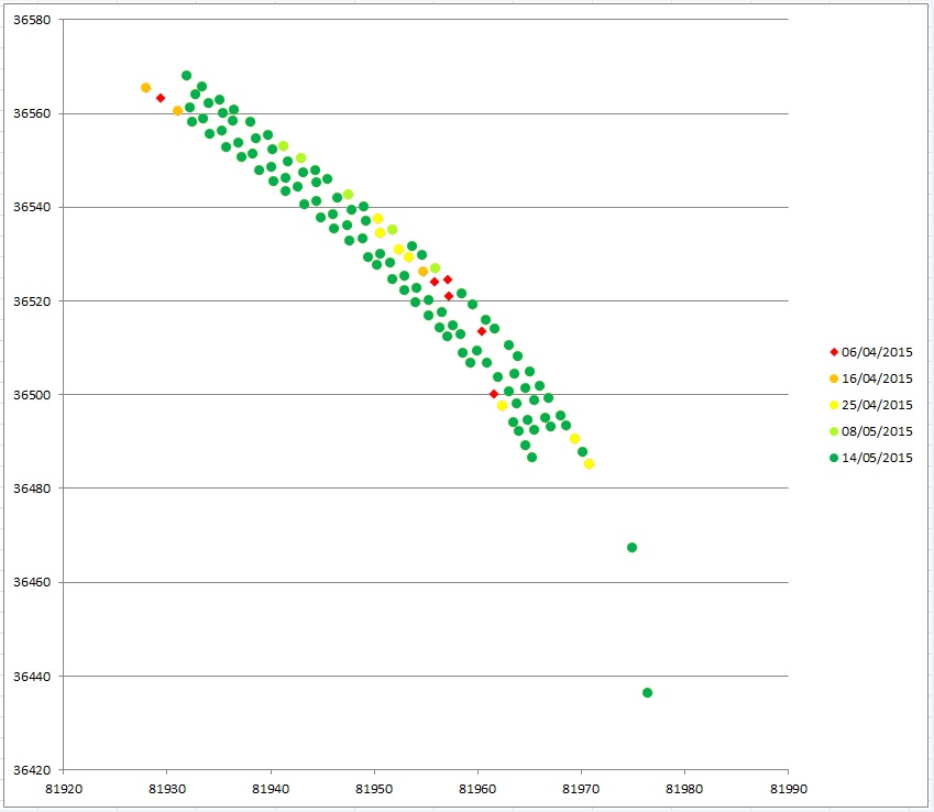
 Track Prism loss mapping
The following figure shows how the prisms are affected in between maintenance rounds. This map has been created based on the April-May gradual prism loss period, and shows how prims stop reflecting the RTS laser in some areas and in most of the cases nearby prisms start behaving in the same way later on. This might suggest that the prism loss in this area is related to prism location, and more precisely, to the reflector’s orientation respect incoming trains.
This theory can be backed with the fact that most of the prisms affected during this period are in the same location as the ones affected during the flooding in January, suggesting that the orientation of those prisms might not be the adequate.
The map also shows that some rails are more prone to contain more vulnerable prisms and will need a more recurrent maintenance than others. In this example the down tracks (on the right hand side) present more issues than the up ones. This can be linked to the presence of a checkrail, more or less adequate orientation, extra brake stress at the front of the train and presence of grease drums on the tracks.
 Conclusion
There are many factors that affect the optical performance of a prism or reflector, but they can be aggravated by a poor installation choice or limiting conditions. That is translated into the need of a more intensive maintenance regime and additional costs. If orientation and/or location of the prisms can be modified after commissioning this could compensate in the long term even if several shifts are required in the first place.
On a big construction interface where there are different constructive episodes the need of a continuous maintenance regime is not always necessary, leading to a system decay between activity episodes. This can lead to network adjustments variations if common or reference prisms are affected by this decay.
The case presented shows how track prisms are logically more vulnerable to optical performance decay whilst structure prisms have almost no variation if they are not interfered with. This should indicate that in order to preserve the system network as stable as possible all critical prisms need to be installed away from the tracks.
-
Authors