Notation

FE, FEA          Finite Element, Finite Element Analysis
FF                    Full Face
MCS                Monitoring Cross Section
SCL                 Sprayed Concrete Lining
SFR                 Steel Fibre Reinforced
TAM                Tube-a-manchette
TBM                Tunnel Boring Machine
TH/B/I              Top Heading/Bench/Invert
VL                    Volume Loss

Introduction

In modern design of complex tunnelling projects it is best practice to utilise 3D finite element analysis (3D FEA), its main advantage being the ability to capture the effects of the actual construction processes and the very influential three dimensional effects. The latter may include the effect of tunnels constructed in close proximity, the interaction with existing structures and the non-homogeneity of the ground conditions. On the other hand, 2D finite element analyses (2D FEA) can be employed for the execution of simplified, quick models which, as long as the engineer is fully aware of the assumptions and the limitations involved, can prove to be a very useful means of calibrating, supplementing and in some cases substituting the demanding 3D models.

An important question at the beginning of a design project is therefore which type of analysis should be applied. As a case example Crossrail’s Farringdon underground station is presented in the following sections. The Crossrail project comprised a combination of long TBM drives forming the running tunnels with sprayed concrete lined (SCL) tunnels forming the station layouts. In principle for such a project, 2D FEA can be used for the design of the running tunnels but inside the footprint of the stations, 3D FEA are necessary for the aforementioned reasons.

There are additional aspects of the design that may need to be considered, such as:

• Sensitivity analyses to assess the weight of several parameters
• Coupled effective stress/pore water pressure analysis
• Consolidation analysis
• Advanced constitutive soil models
• Advanced concrete models
• Excavation sequence (ie exact simulation of face divisions for SCL tunnels)

However, realistically these cannot all be incorporated in a 3D FEA due to the limited time frames and resources.

The following sections present a combination of 3D and 2D FEA that has been used to back analyse the actual performance of the SCL tunnels. The findings of this exercise as well as the importance of the inverse analysis in tunnel design are highlighted in the context of practical FE modelling.

The role of Inverse Analysis

Inverse or back analysis is a commonly used practice in civil engineering, widely applied in slope stability problems and could be defined as the execution of an analysis (finite element, limit equilibrium etc.) where the problem parameters are varied accordingly until a known result is derived. These parameters that lead to the correct (or known) solution are considered as ‘back analysed’ and the model as accordingly calibrated.

A good example on the application of the back analysis with respect to the 3D effects in slope stability problems comes from Duncan and Wright^[2]. A slope stability problem is in most cases analysed using 2D limit equilibrium analyses (or/and FEA) where a factor of safety is calculated. This approach though excludes the very important 3D effect, ie the geometrical characteristics of the slope and the side shear (ratio width/length). In a normal analysis, excluding these factors would result in the calculation of a conservative factor of safety. However, in a back analysis (where the slope has failed and the factor of safety is unity), exclusion of the 3D effects would result in high soil parameters along the slip plane, therefore in an non-conservative assessment.

Similar considerations are valid for tunnel design. Inverse analysis in tunnelling projects can be performed by varying parameters appropriately in order to derive the deformations observed through in-tunnel or surface level monitoring. The parameters that can be varied in a finite element model may include the strength/stiffness of the soil or concrete, the simulation steps, the geometry of the finite elements mesh etc.

Two very important aspects that the authors would like to make note of are:

• The parameters should vary within a natural range.
• The back analysis should not aim to either a conservative or non-conservative solution, but simply should try to replicate the actual behaviour as closely as possible.

Case Study: Crossrail Farringdon Station

Farringdon station will provide interchange between Crossrail, London Underground and Thameslink rail networks. During its construction, an important role that the station had was the reception of the two Drive X and the two Drive Y TBMs as shown in Figure 1.

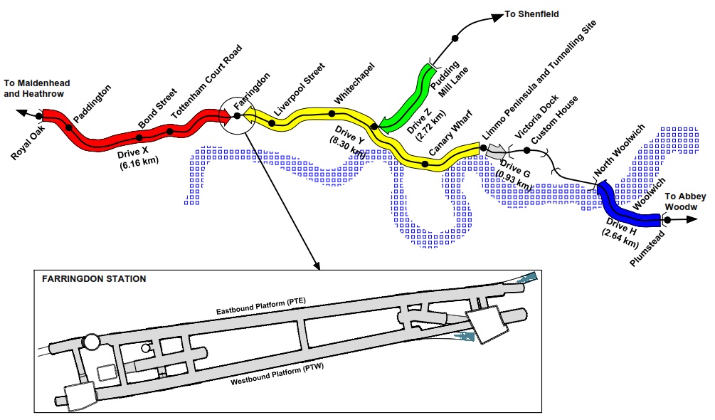
Figure 1 – Crossrail route with focus on Farringdon Station.

The station was constructed at approximately 30m below street level and comprised 2 ticket halls that provided connection to the platform level via 2 escalator inclines with subsequent concourse tunnels, two platform tunnels enlarged from the already constructed TBM tunnels, approximately 300m long each, and multiple cross passages and ventilation tunnels. The main contractor Bam, Ferrovial, Kier joint venture (BFK), was awarded the contract (C435) by Crossrail Ltd. BFK employed Dr Sauer & Partners (DSP) as their SCL specialist.

Two special features related with Farringdon Station were:

• The construction phasing of the platform tunnels: they were enlarged using SCL methods from the existing TBM tunnels.
• The tunnels were constructed mainly in the Lambeth Group formation, a mixture of very stiff over consolidated Clays which constituted an excellent open face tunnelling medium with the exceptions of the interbedded sand lenses with water pressures that added a certain level of difficulty and risk to the SCL tunnelling operations.

In-tunnel Monitoring Analysis

The deformations of the approximately 1 km of SCL tunnels in Farringdon station were monitored using a high precision total station to survey monitoring targets. These targets were installed at predefined monitoring cross sections (MCS) generally spaced every 10m. The typical layout of a platform tunnel monitoring cross section is shown in Figure 2. Absolute deformations of each target were acquired on a daily interval following the construction of the tunnel section at that chainage.

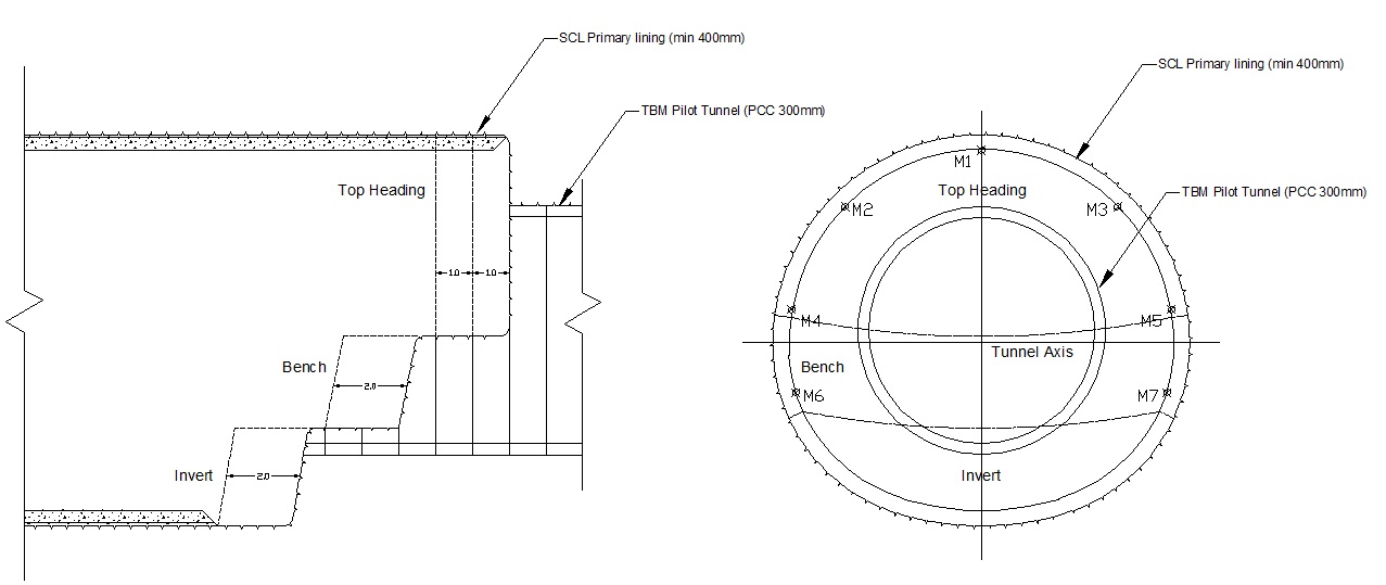
Figure 2 – Typical excavation and support sequence showing the typical layout of a monitoring cross section. The platform tunnel was 11.35m wide by 10.66m high (excavation line).

Three phases can be distinguished in a typical time plot of the in-tunnel deformations as shown in Figure 3 :

• The initial deformation phase starts with the first readings and lasts for 3 to 5 days, exhibiting almost linearly increasing deformations with time.
• The levelling out phase starts with the ring closure, where the in-tunnel deformations clearly start levelling out and lasts for another 3 to 5 days.
• The stable phase then follows where in the absence of subsequent tunnel excavation in the proximity, only minor fluctuations of the readings are expected. These fluctuations are not related to actual lining deformation but are a result of other factors such as the monitoring accuracy, temperature changes, construction vibrations etc.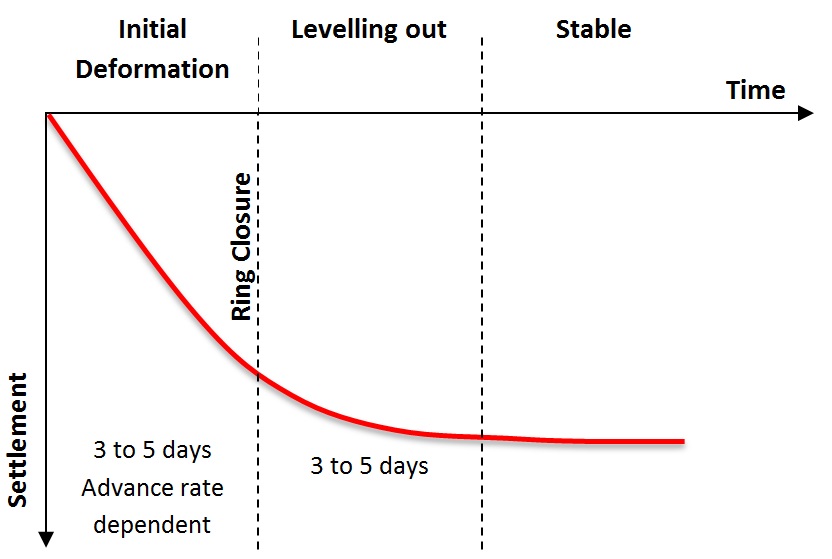

Figure 3 – Typical phases in a time plot of the in-tunnel deformations.

A very dense network of compensation grouting arrays (tub-a-manchettes or TAMs) was installed in Farringdon, covering a large portion of the station’s footprint. In order to exclude the effect of compensation grouting in this paper, the average in-tunnel deformations of the parts of the two platform tunnels (Eastbound and Westbound) that were not covered by TAMs were derived and summarised in Table 1 below.

3D FE Design Models

For computational efficiency reasons, a decision was made to divide the temporary SCL tunnels in Farringdon into separate, smaller 3D FE models. The four main models are shown in Figure 4, namely the West ticket hall area model, the East ticket hall area model, the SCL access shaft area model and the triple connection to the East ticket hall.

These individual models were created to address and tackle particular design issues and challenges. Three dimensional modelling provided an opportunity to consider the 3D effects of tunnelling in the course of construction, ground/structure interaction, face stability deriving information regarding volume loss and ground movement without subjective assumptions.

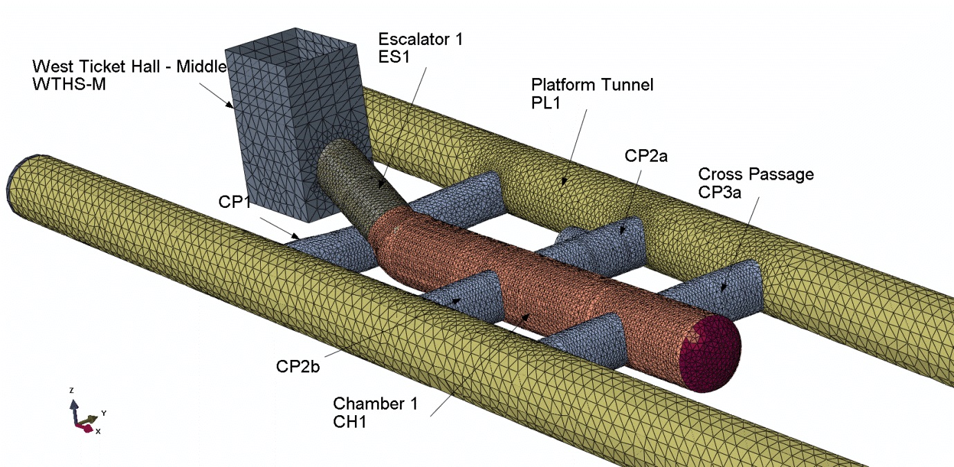
(a) West Ticket Hall area	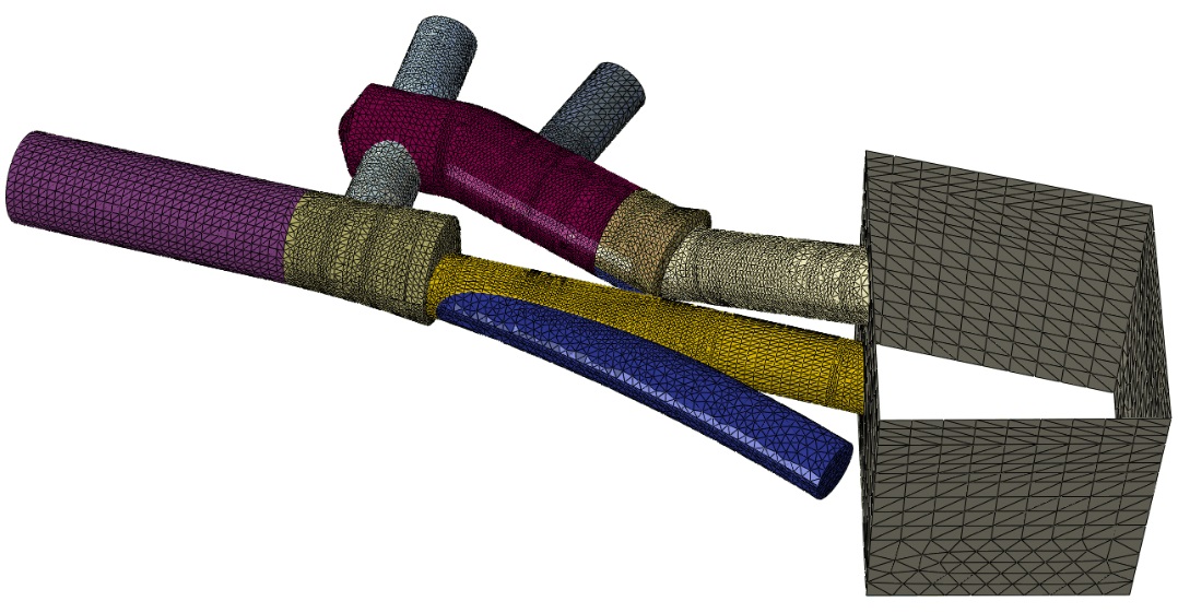(b) West Ticket Hall area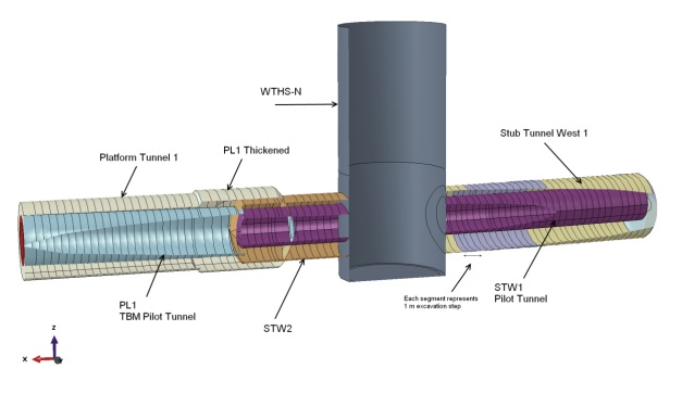
(c) West Ticket Hall area	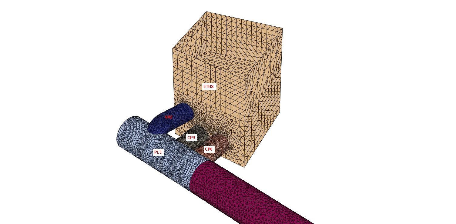(d) West Ticket Hall area
Figure 4 – Main 3D FE design models across the Crossrail Farringdon Station.

The purpose of the 3D FE design analyses in this project was to dimension the lining thickness at complex situations (e.g. triple junction, close proximity to other tunnels etc.), to optimise the temporary works excavation sequences and providing trigger values for monitoring purposes.

ABAQUS Version 6.12 (Dassault Systemes Simulia)^[1] a general purpose finite element software package was used to perform the numerical analyses. Soil materials were modelled with the elastic-perfectly plastic Mohr-Coulomb model. For the purpose of the primary SCL design no groundwater pressure was applied in the analysis since the primary lining is not considered to be watertight. Undrained soil parameters were taken for the analysis in order to account for the “fast” construction in comparison to the time of consolidation in the London Clay. The numerical analyses have been undertaken on the basis of a total stress analysis. Both undrained shear strength (Cu) and Young modulus (Eu) of the clay stratums increased linearly with depth.

Additionally, two main characteristics of the geology in Farringdon, the presence of the faults and the variation of the thickness of the London Clay, have been simulated in the models.

The fibre reinforced sprayed concrete (SFRC) was modelled as a linear elastic – perfectly plastic material considering the post failure material behaviour determined by residual flexural tensile strength of SFRC.

In all the models, the simulation of the sequential excavation and lining installation followed a multi-step analysis based on the designed excavation and support sequences. The excavation and lining installation of one advance was performed in two steps; i.e. the soil was removed in the first step and the lining was installed in the second step.

All the major excavation sequences (Top heading, bench & invert) in large tunnels such as platform and concourse tunnels were simulated according to the drawings while in small size tunnels (e.g. cross passages) a full face method was considered.

Back Analysis optimisation

Both 2D and 3D FEA were used to perform inverse analysis. The main scope of the 3D FE back analyses was to assess the effect of the type of the simulation of the excavation, ie between a full face excavation and the actual division of the face in top heading, bench and invert.

For this purpose, a more simplified 3D model (Figure 5a) was constructed where one platform tunnel was excavated following various excavation sequences, namely:

– Two top headings, bench, invert (TH-B-I)
– Two top headings, invert, bench (TH-I-B)
– Two top headings, combined bench and invert (TH-B+I)
– Full face (ie 1m rings)

All top heading steps were 1m long and all Bench/Invert excavation steps were 2m long.
The first important conclusion was that the difference between the TH-B-I, TH-I-B and TH-B+I simulations was minor, therefore the simpler TH-B+I simulation was used instead.
A simplified 2D FE model (Figure 5b) was also constructed in order to assist in the multiple back analyses.

The general steps of the simulation were the following:

1. Geostatic stress state
2. Softening of subsequently excavated TBM tunnel area by 50%
3. Installation of TBM lining and removal of softened soil
4. Simulation of the stepwise excavation of the Platform tunnel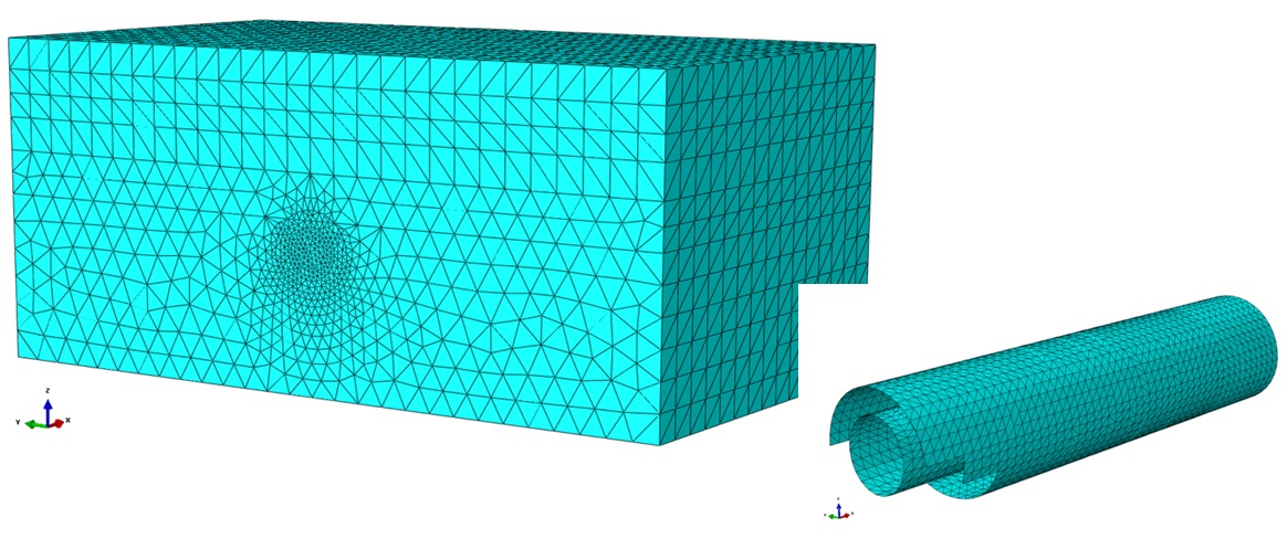

a. 3D FE back analysis model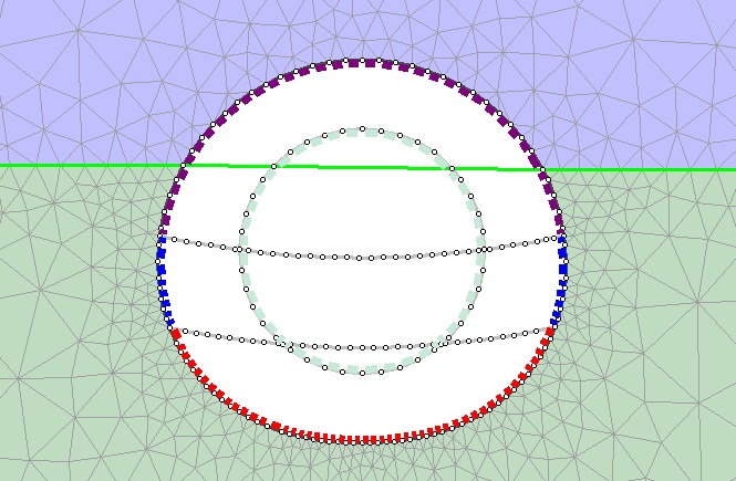

b. 2D FE back analysis model

Figure 5 – 3D and 2D models used for the back analyses.

Comparisons

The calibration of the back analysis models assumed the following 3 factors:

– Predict the in-tunnel displacements as accurately as possible
– Predict the surface settlements as accurately as possible
– Avoid underestimating the lining stresses

For the in-tunnel displacements comparison, the average values as shown in Table 1 were used.

Figure 6 shows the results for 2 different values of the earth coefficient at rest (ko) of the 3D FE design models (FF k_o=0.6 and FF k_o=1.2 where FF denotes Full Face), the back analysis 3D models (TH-B+I k_o=0.6 and k_o=1.2) and the 2D FE back analysis models.

It is shown that the analyses with k_o=1.2 overestimated the transverse displacements and underestimated the vertical displacement of the crown. Both the 3D FEA with TH-B+I excavation and the 2D FEA with k_o=0.6 showed an excellent match with the in-tunnel displacements. Similar results have been presented in ^[3], ^[4],

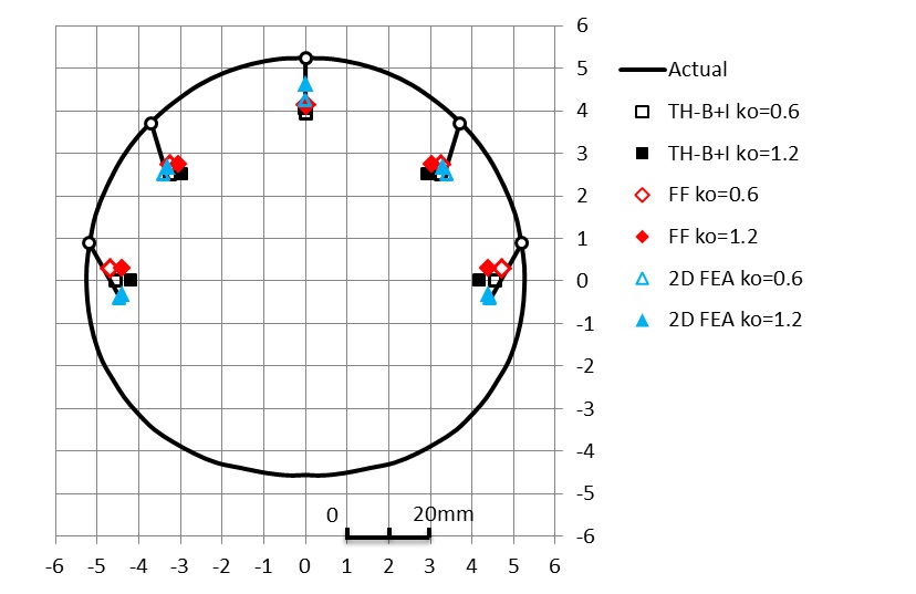
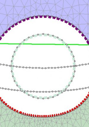
Figure 6 – Comparison of the actual average and the predicted in-tunnel deformations.

For the comparison of the surface settlements, one of the very few continuous monitoring arrays where no compensation grouting was carried out was chosen. The accuracy of the models with k_o=0.6 as compared to the ones with k_o=1.2 is shown in Figure 7. Although the actual performance of the surface was very stiff, possibly affected by the existing foundations, the 3D and the 2D FE model with k_o=0.6 produced more satisfying settlement troughs, which correspond approximately to a volume loss between 0.4 and 0.5%. These values correspond only to the enlargement from the existing TBM tunnels using SCL methods, thus excluding the volume loss induced by the TBM excavation.

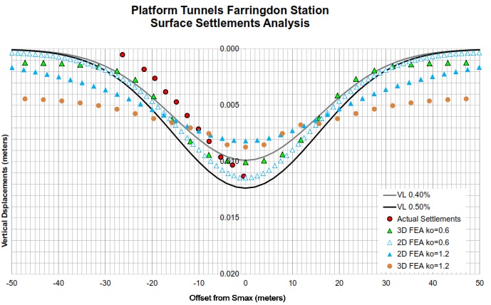
Figure 7 – Comparison of the actual and the predicted transverse settlement troughs. Different volume loss curves are also shown.

Conclusions

From the 3D and 2D FEA that were utilised to perform the back analyses in Crossrail Farringdon station, the following important conclusions could be drawn:

– The prediction of the surface settlement is very sensitive to the k_o value.
– In a 3D FE analysis, the division of the excavation sequence in Top Heading, Bench and Invert produces similar results in-tunnel displacements and lining stress results if the bench and the invert are combined into one step.
– Both 3D FE analyses simulating a full face excavation (FF) and a divided TH/B/I excavation produce very similar settlement troughs. For this purpose, the more simplified FF simulation can be used.
– For the ground conditions in Farringdon station, a value of ko=0.6 produced more realistic deformation results (in-tunnel and surface settlements).
– The volume loss attributed solely to the SCL enlargement of the Platform tunnels from the existing TBM tunnels in Farringdon, varied between 0.4% and 0.5%.
– The 2D FE back analysis, predicted both in-tunnel and surface settlements very reliably. This was expected at some extent as the spans of the platform tunnels between junctions were long enough to be able to approximate plain strain conditions.

Simple 2D or/and 3D calibration models can be utilised in order to derive similar valuable information that may increase the performance and reliability of large scale 3D FE models.

References

[1] Dassault Systemes Simulia 2011. ABAQUS Analysis User’s Manual-V6.12.
[2] Duncan, J.M. & Wright, S.G. 2005, Soil strength and slope stability, John Wiley & Sons.
[3] Gakis, A., Flynn, S. Nasekhian, A. 2014. Back analysis of observed measurements for optimised SCL tunnel design. North American Tunnelling: 2014 Proceedings.
[4] Gakis, A. 2014. Design of a SCL wraparound tunnel utilising a 3D geological model for Crossrail Farringdon Station. BTS Harding price 2014 finalist paper. (please see in www.britishtunnelling.org.uk).