Design of the Deep Cut and Cover Crossrail Paddington Station Using Finite Element Method
Document
type: Technical Paper
Author:
Mitesh Chandegra MEng MSc MICE CEng, Aliki Kokkinou Diploma MSc & DIC, ICE Publishing
Publication
Date: 31/08/2016
-
Read the full document
Nomenclature
CAU Anisotropically consolidated undrained triaxial compression and extension tests with mid-height and base pore pressure and local axial and radial strain measurement CIU Isotropically consolidated undrained triaxial compression and extension tests with mid-height and base pore pressure and local axial strain measurement cincr Cohesion increase with depth cref Cohesion (constant) dinter Equivalent thickness of the interface elements DR Departures Road EA Normal stiffness of the plate element EBT Eastbourne Terrace Road EI Flexural rigidity of the plate element 
Elastic modulus based on triaxial tests (secant stiffness) used in Hardening soil model and defined for a reference stress level Einc Elastic modulus increasing with depth used in Mohr Coulomb soil model 
Elastic modulus based on oedometer tests (tangent stiffness) used in Hardening soil model and defined for a reference stress level E’ Elastic modulus used in Mohr Coulomb soil model and defined for a reference elevation level 
The initial elastic modulus at very small strain and defined for a reference elevation level 
Elastic modulus for unloading and re-loading conditions used in Hardening soil model and defined for a reference stress level FE Finite Element 
Reference shear modulus at very small strain HS Hardening soil model HSS Hardening soil model with small strain stiffness K0nc Coefficient of lateral pressure at rest for normally consolidated soils kx Permeability in horizontal direction ky Permeability in vertical direction m Value used to identify the variation of elastic modulus with depth for the Hardening soil model MC Mohr-Coulomb model pref Confined reference stress value corresponding to elastic modulus. Rf Percentage defining the failure asymptote for stress-strain curve Rinter Reduction factor for reducing the shear strength parameters of the soil in contact with structures. s Bored Pile Spacing TStrength Tension stress in the material. UUP Unconsolidated undrained triaxial compression tests with mid-height pore pressure and local axial strain measurement CAU Anisotropically consolidated undrained triaxial compression and extension tests with mid-height and base pore pressure and local axial and radial strain measurement CIU Isotropically consolidated undrained triaxial compression and extension tests with mid-height and base pore pressure and local axial strain measurement W Weight yref Depth reference to where material (strength) parameters increases with depth for Mohr-Coulomb model Φ Friction angle σt Tensile cut off γ0.7 Shear strain magnitude at 0.722G0 γsat Saturated bulk density γunsat Unsaturated bulk density ν Poisson’s ratio vur Poisson’s ratio of the material for unloading-reloading ψ Angle of dilatancy of the material Introduction
The deep cut and cover Crossrail Paddington Station is constructed in one of London’s most significant existing transport hubs, primarily through London Clay. The two-dimensional finite element software Plaxis 2D was used for the design, which was undertaken in accordance with Crossrail Civil Engineering Design Standards Part 3 CEDS-3[8] .
The undrained behaviour needs to be considered for London Clay. Using the software Plaxis, this behaviour can be assessed in two ways; in terms of effective and total stresses. There are three constitutive ground models commonly used for such analyses; Mohr-Coulomb model, Hardening soil model and Hardening soil model with small strain stiffness. A comparison of the results of the FE models with the measured wall deflections, derived from inclinometers located within and behind the main box diaphragm walls, can give a useful insight on the performance of the geotechnical design.
It should be noted that each of these models requires different input parameters, the influence of which on the outcome of the analysis is of interest.
The evaluation of the performance of the diaphragm wall modelling is expected to be helpful to engineers and researchers that need to perform similar analyses, allowing them to use these models with more confidence.
The Site
The Crossrail Paddington Station is the most westerly underground station of Crossrail, located directly beneath Departures Road and Eastbourne Terrace, aligned with the existing Grade I listed Paddington mainline station. The location of the new station and the constraints from the surrounding buildings, among which are the Grade 1 Mainline Station, Macmillian House and the Hilton Hotel, are presented in Figure 1.
The station is a deep cut and cover underground box structure approximately 264 m long, 24 m wide and 24 m deep, framed with 40 m long diaphragm walls of 1200 and 1000 mm thickness installed along the box perimeter down to 85.5 m ATD. The general excavation depth is around 21 m below Departures Road and 24 m below Eastbourne Terrace. A top-down construction has been adopted, using plunge columns that are connected to 1800 mm diameter and 40m long bored piles along the centreline of the box. These piles initially carry the temporary construction loads from the upper floors on the plunge columns and subsequently support the permanent columns and resist the long term uplift forces. Four permanent slabs prop the diaphragm wall panels during construction and in the permanent case. Figure 2 shows a typical cross section through the station.
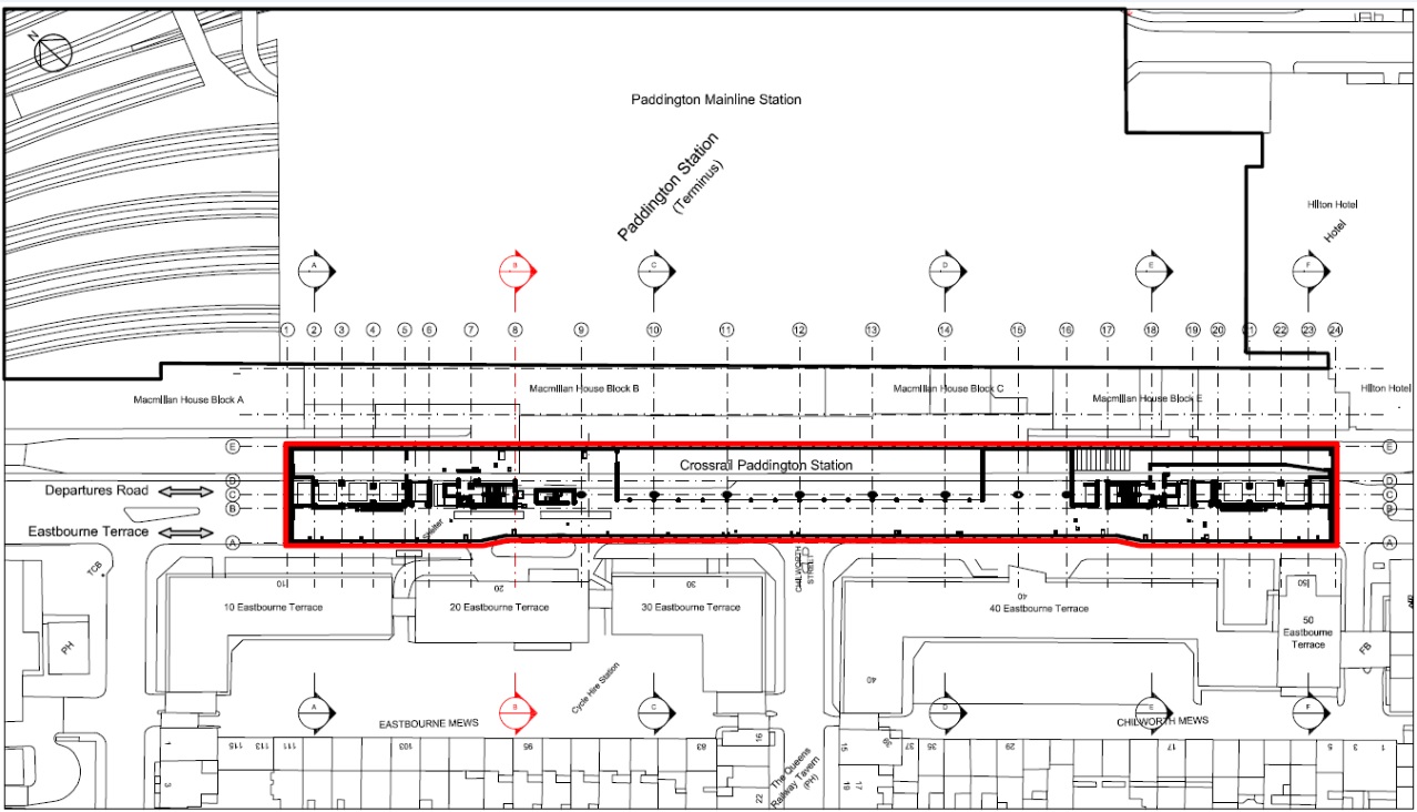
Figure 1 – Location Plan view of Crossrail Paddington Station 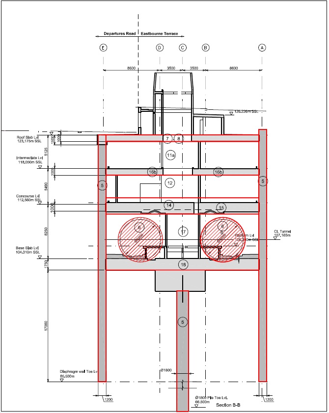
Figure 2 – Typical Cross section of Paddington Station Geological Profile
The site is underlain by Made Ground, and occasionally Langley Silt, overlying in turn by River Terrace Deposits and London Clay of significant thickness, over the Lambeth Group, followed by the Upnor Formation, Thanet Sand and Chalk. The entire Paddington Crossrail construction does not penetrate the base of the London Clay. There are two aquifers beneath the site; a shallow upper aquifer in the River Terrace Deposits and a lower deep aquifer in the Chalk, Thanet Sand and Upnor Formation.
Analysis and Results
Design Approach
Plane strain finite element analysis of the Paddington main station box has been performed using the FE package Plaxis 2D (version 9.02), with 15 node elements and medium mesh coarseness with local mesh refinement.
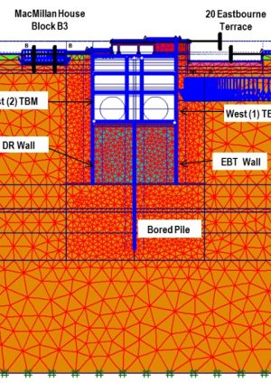
Due to variation in the station box layout and adjacent existing structures, six different sections have been identified for the analysis. The location of these sections, named Sections A to F, along the box is shown on Figure 1. This paper focuses solely on Section B, which is adjacent to 20 Eastbourne Terrace and MacMillan House Block B. The rigidity of both these existing structures was accounted for by modelling fixed end anchor props with high stiffness at the top of the basement levels. A typical FE model section is shown in Figure 3.
The analysis has been carried out in accordance with CEDS-3[8] for the modelling of the initial and long-term conditions, thus assuming drained conditions when simulating the initial conditions and the design life situation of the station box accordingly. For the modelling of the excavation and the construction stages of the box a different approach from the original analysis has been adopted. The original analysis was modelled with drained conditions on the active and undrained conditions on the passive side, in line with the CEDS-3. However, fully undrained conditions throughout the model have also been considered for the design analysis. A comparison between the two different approaches is discussed later.
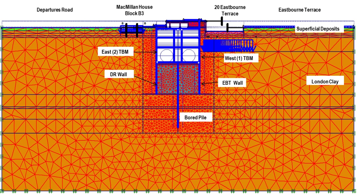
Figure 3 – Typical FEA Cross section The Ground Constituent Models
The Mohr-Coulomb, Hardening Soil and Hardening Soil with Small Strain Stiffness models can be simulated as either drained or undrained. The excavation problem is mainly influenced from the undrained behaviour of London Clay and therefore the three constitutive soil models were adopted to simulate the undrained conditions in order to evaluate their performance in predicting the wall deflections.
The soil models are merely an approximation of the real soil behaviour and thus it is important to consider their inherent assumptions and limitations when applied [3]. An example of incorrect use of the soil models is best illustrated in the Nicoll Highway collapse [9].
Mohr Coulomb model (MC)
The Mohr-Coulomb model represents a first order approximation of soil and rock behaviour, assuming the stress-strain relation to be linear elastic-perfectly plastic. The slope of the linear elastic section of the stress-strain curve is defined as the Young’s modulus of soil (E’), and the perfectly plastic section is obtained when the stress states reach the Mohr-Coulomb’s failure criterion.
An increase in soil stiffness with depth can be modelled. However, the model does not account for stress dependency, stress-path dependency of stiffness or anisotropic stiffness [4].
The MC model involves six input parameters (c, φ, Ε’, v, ψ, σt). The effective friction angle (φ) for London Clay was directly obtained from laboratory tests. Effective cohesion (c) was assumed to be zero, but to aid computation in the calculations of PLAXIS, a very small value c = 1 kPa was adopted. The drained Poisson’ ratio was assumed to be 0.2.
![Figure 4 - Mohr-Coulomb Soil Model[4]](https://learninglegacy.crossrail.co.uk/wp-content/uploads/2016/11/7E-008-Figure-4.jpg)
Figure 4 – Mohr-Coulomb Soil Model[4] Hardening Soil Model (HS)
The Hardening Soil model is an advanced soil model that has a hyperbolic stress-strain relationship and uses the same failure criterion as the MC model. The hyperbolic stress-strain relation between the axial strain ε1 and deviatoric stress q for primary loading is presented in Figure 5 and defined by Equations (1) and (2)[4].
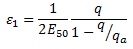
(1) 
(2) Rf
where qa is the asymptotic value of the shear strength; qf is the failure value derived from the Mohr Coulomb criterion; Rf is the failure ratio, which is taken as 0.9; and E50 is the confining stress-dependent stiffness modulus for primary loading. This is defined by Equation (3).
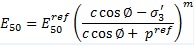
(3) where
 is a reference stiffness modulus corresponding to the reference confining pressure, pref;
  is the minor principal stress; and m is the stress dependence power, which is recommended to be close to 0.5 for sands and 1.0 for soft clays in the Plaxis manual[4].
The stress dependent stiffness for the loading and unloading stress paths is defined by Equation (4).
 is recommended to be used in the Plaxis manual[4].
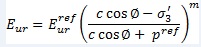
(4) The HS soil stiffness is calculated, using three different reference stiffness parameters; triaxial loading secant stiffness E50 , triaxial unloading/reloading stiffness Eur and oedometer loading tangent stiffness Eoed. These three moduli are defined at a reference stress level pref, and power m for the stress dependent stiffness formulation. Typically pref is taken as 100 kPa.![Figure 5 - Hyperbolic Curve for Hardening Soil Model [4]](https://learninglegacy.crossrail.co.uk/wp-content/uploads/2016/11/7E-008-Figure-5.jpg)
Figure 5 – Hyperbolic Curve for Hardening Soil Model [4] Unlike the MC model, which represents soil stiffness in the in-situ stress state, the HS model does account for stress-dependency of the stiffness moduli (soil stiffness increases with stress). However, it does not distinguish between large stiffness at small strains and reduced stiffness at engineering strain levels.
The HS is better suited to model excavation problems compared to the MC model due to its ability to model the unload-reload stiffness. The MC model is based on elastic behaviour and thus it is unable to model density and shear hardening, potentially making it inaccurate for deformation problems.
The HS model is an isotropic hardening model, so does not account for hysteretic, cyclic loading or cyclic mobility. The model does not account for soil softening due to soil dilatancy and de-bonding effects [4].
There are 10 input parameters for the HS model. The parameters of c, φ, v, ψ and σt are the same as those used in the MC model.
Hardening Soil Model with Small Strain Stiffness (HSS)
Hardening Soil model with small strain is a modification of the HS model that accounts for the small strain characteristics of soil, based on the research of Benz[2]. More specifically, the stiffness varies non-linearly with strain, being higher at low strain levels compared to the strains associated with general construction works (Figure 6).
The HSS model uses a modified hyperbolic law for the stiffness degradation curve, which was proposed by Hardin and Drnevich[11] and Santos and Correia[13]. In addition to the parameters adopted for the HS model, the HSS model requires two additional parameters (i.e. 12 input parameters in total), which are the reference shear modulus at very small strain (G0ref) and shear strain (γ0.7) at which the secant shear modulus is equal to 72.2% of its initial shear modulus value (G0).![Figure 6 - Stiffness Strain Behaviour[4]](https://learninglegacy.crossrail.co.uk/wp-content/uploads/2016/11/7E-008-Figure-6.jpg)
Figure 6 – Stiffness Strain Behaviour[4] Undrained Analysis
Analysis of the undrained conditions can be conducted by either using an effective stress or total stress approach. In the effective stress analysis water and soil are treated separately, whereas in the total stress analysis water and soil are treated as a single material. The undrained state can be modelled using the following three approaches:
Undrained (A): Undrained effective stress analysis with effective shear strength parameters
- Effective strength parameters c, ϕ, ψ
- Effective stiffness parameters E’, ν
- Allows for change of strength with change in effective stress (due to loading, unloading or water pressures).
- Required for utilising features of both the HS and HSS models
Undrained (B): Undrained effective stress analysis with undrained shear strength parameters
- Undrained total strength parameters c = Cu, ϕ = 0, ψ = 0
- Effective stiffness parameters E’, ν
- Its main limitation is that change in effective stress will not result in change of the soil strength.
- The HS and HSS models involve frictional hardening characteristics to model plastic shear strain in deviatoric loading, and cap hardening characteristics to model plastic volumetric strain in primary compression. However, with ϕ =0 the stiffness moduli of the model is no longer stress dependent and exhibits no compression hardening, despite retaining shear hardening and unloading-reloading modulus.
Undrained (C); Undrained total stress analysis with undrained shear strength parameters:
- Undrained total strength parameters c = Cu, ϕ = 0, ψ = 0
- Total stiffness parameters Eu, νu = 0.495
Ideally, effective stress analysis and thus Undrained (A) modelling is recommended. However, if information on effective strength parameters is not available and since the total stress parameters are easier to be obtained with conventional soil tests, Undrained (B) modelling could be adopted.
Care should be taken in simulating undrained conditions with Undrained (A) since the effective stress path that is followed may not be realistic, particularly for normally consolidated soils[11]. As shown in Figure 7, if the Undrained (A) approach is selected, the MC model can overestimate the undrained shear strength due to the elastic-perfectly plastic assumption.
The conversion between undrained strength (Cu) and effective strength parameters (φ and c) should always be checked to ensure that the adopted parameters are reasonable. Based on the effective stress path for undrained plane strain shearing using Mohr-Coulomb soil model the undrained stiffness is defined by Equation (5).![Figure 7 - Illustration of stress path; Reality vs MC Model[11]](https://learninglegacy.crossrail.co.uk/wp-content/uploads/2016/11/7E-008-Figure-7.jpg)
Figure 7 – Illustration of stress path; Reality vs MC Model[11] 
(5) As no distinction is made between effective stresses and pore pressure it is not recommended to use the Undrained (C) approach for advanced soil models and it has not been considered further.
Refer to Plaxis Material Models Manual [4] for further discussion on the interpretation of the undrained approaches.
Design Soil Parameters
The Plaxis input design soil parameters are presented in Table 1. The model parameters for London Clay are provided for the Undrained (A) approach. For the Undrained (B) Approach, the soil strength was defined by Cu=85+5z, where z is equal to 0 at 120 m ATD.
The effective stiffness with depth, equivalent to 750Cu, was adopted for the MC model. This together with the HS model
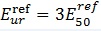
profile is presented in Figure 8. The unload/reload stiffness,  , was assumed to be equal to 3
 . The small strain Young’s modulus
  was conservatively adopted to be equal to , based on the chart by Alpan[1]. The shear modulus was subsequently determined based on the following expression:
(6) The γ0.7 was estimated using the following suggestion in the PLAXIS manual:
(7) Table 1– Characteristic Soil Parameters Summary
Parameter Name Units Made Ground Terrace Gravel Light Weight Fill London Clay London Clay London Clay Material model – – Hardening Soil Hardening Soil Hardening Soil Mohr Coulomb Hardening Soil Small Strain Hardening Soil Type of material behaviour – – Drained Drained Drained Undrained (A) Undrained (A) Undrained (A) Dry soil weight γsat [kN m-3] 18 20 12 20 20 0 Wet soil weight γunsat [kN m-3] 18 20 12 20 20 0 Permeability in hor. Direction k_x [m/day] 8.64E-06 8.64E-06 8.64E-06 8.46E-06 8.46E-07 8.46E-07 Permeability in vert. direction k_y [m/day] 8.64E-06 8.64E-06 8.64E-06 8.46E-06 8.46E-07 8.46E-07 Secant stiffness in standard drained triaxial test [kN m-2] 10000 60000 20000 – 77625 77625 Tangent stiffness for primary oedometer loading 
[kN m-2] 10000 60000 20000 – 77625 77625 Unloading/reloading stiffness [kN m-2] 30000 180000 60000 – 232875 232875 Young’s Modulus stiffness E’ [kN m-2] – – – 77625 – – Young’s Modulus Increment [kN m-2] – – – 3750 – – Cohesion cref [kN m-2] 20 1 1 1 1 1 Friction angle φ [ ° ] 25 36 37 24 24 24 Dilatancy angle ψ [ ° ] 0 0 0 0 0 0 Poisson’s ratio for unloading/reloading νur [ – ] 0.2 0.2 0.2 0.2 0.2 0.2 Reference stress for stiffness pref [kN m-2] 8 15 8 – 100 100 Power for stress-level dependency of stiffness m [ – ] 0.01 0.01 0.01 – 0.6 0.6 Ko value for normal (1 – sin φ′, default setting) K0nc [ – ] 0.577 0.41 0.398 0.593 0.593 0.593 Lateral Coefficient of At Rest Earth Pressure, Ko K0 [ – ] – – – 1.0 1.0 1.0 Cohesion Increment cincr [kN m-3] 0 0 0 0 0 0 Cohesion and stiffness reference level yref [m] 0 0 0 116.3 0 0 Failure ratio (default setting) Rf [ – ] 0.9 0.9 0.9 0.9 0.9 0.9 Tensile Cut of Stress value σt [kN m-2] 0 0 0 0 0 0 Interface strength reduction factor Rinter [ – ] 0.67 0.67 0.67 0.67 0.67 0.67 Reference small strain shear modulus 
[kN m-2] 139725 Shear strain magnitude at 0.722G0 γ0.7 [ – ] 0.000293 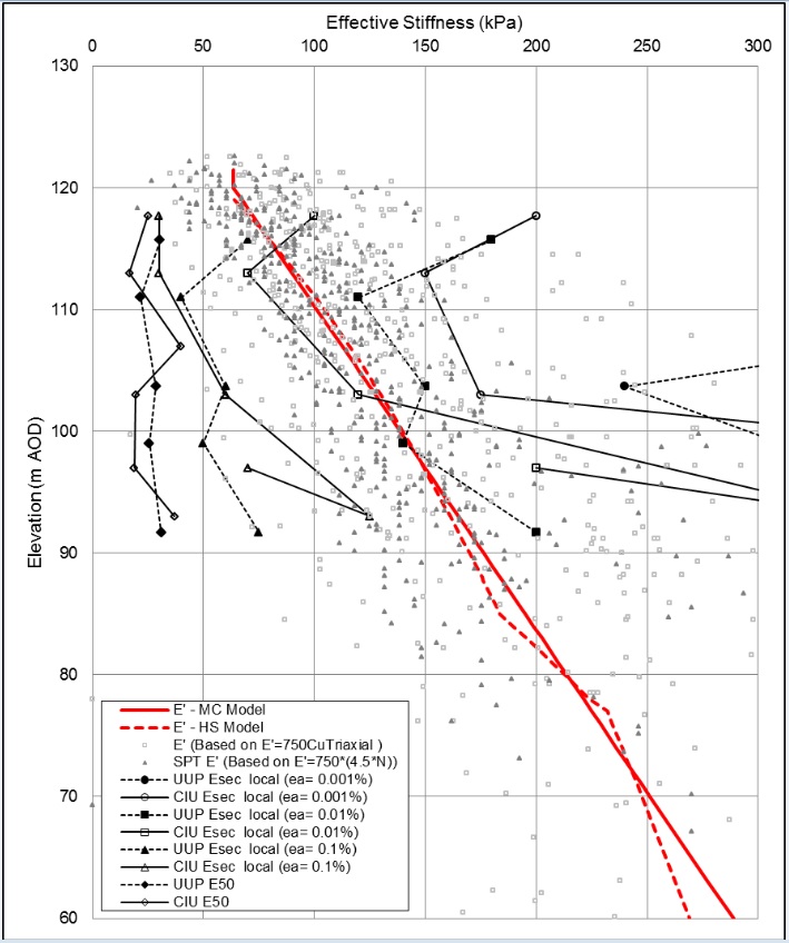
Figure 8 – Effective Stiffness with depth Structural Elements
The diaphragm walls, columns, piles and floor slabs have been simulated by plate elements, the characteristics of which are presented in Table 2 to Table 6. The short term and long term stiffness properties of the concrete elements were reduced by 30% and 50%, respectively, from their nominal values to consider the cracking and creep in the diaphragm wall and slabs due to bending.
To account for the dimensions of the floor slabs and the various voids within them, the properties of the plate elements were adjusted along their unit length. An example of how the floor properties are determined is presented in Figure 9 and Table 6.
Table 2 – Properties of 1200mm Diaphragm Walls
Parameter Name Unit Value Compressive strength of concrete f’c MPa 35 Young’s modulus E MPa 34077 Thickness d M 1.2 Axial stiffness x 70% 70%EA MN/m 28625 Flexural stiffness x 70% 70%EI MNm2/m 3435 Axial stiffness x 50% 50%EA MN/m 20446 Flexural stiffness x 50% 50%EI MNm2/m 2454 Weight W kN/m/m 16.80 Poisson’s ratio ν 0.2 Table 3 – Properties of 1800mm Diameter Bored Pile at 5500mm centres
Parameter Name Unit Value Compressive strength of concrete f’c MPa 35 Young’s modulus E MPa 34077 Thickness d m 1.2 Axial stiffness x 70% 70%EA MN/m 11037 Flexural stiffness x 70% 70%EI MNm2/m 2235 Axial stiffness x 50% 50%EA MN/m 7883 Flexural stiffness x 50% 50%EI MNm2/m 1596 Weight W kN/m/m 6.48 Poisson’s ratio ν 0.2 Table 4 – Material Properties for Plunge Columns
Parameter Name Value Unit Elastic Modulus E E 210000 MN/m2 Axial stiffness EA/s 3649 MN/m Flexural stiffness EI /s 182 MNm2/m Weight W 1.20 kN/m Poisson’s ratio ν 0.2 Table 5 – Material Properties for elliptical concrete columns
Parameter Name Value Unit Axial stiffness EA/s 1631 MN/m Flexural stiffness EI /s 136 MNm2/m Weight W 1.20 kN/m Poisson’s ratio ν 0.2 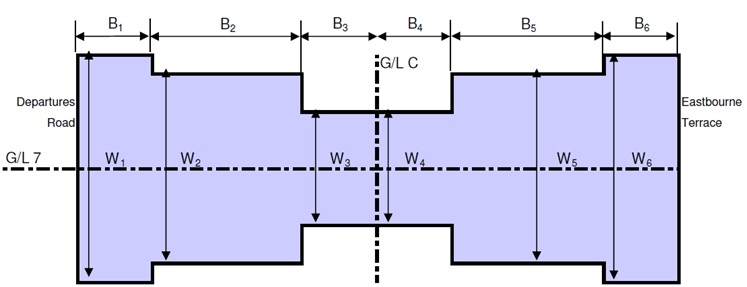
Figure 9 – Plan view of Roof Slab Table 6 – Properties of Floor Slabs
Parameter Symbol Units Slab No. Section – – B1 B2 B3 B4 B5 B6 Length B (m) 3 5.3 3.35 2.7 – 8.95 Width W (m) 10.8 5.75 3.35 1.78 – 10.8 Depth T (m) 1 1 1 1 – 1 Axial stiffness x 70% EA (MN/m) 24654 13126 7647 4063 – 24654 Flexural stiffness x 70% EI (MNm2/m) 2055 1094 637 339 – 2055 Weight W KN/m 24 12.78 7.44 3.96 – 24 Poisson’s ratio ν 0.2 0.2 0.2 0.2 – 0.2 The floor slab/ wall connection can be modelled in four ways, as shown in Figure 10. By using volume elements, the floor slab geometry and material properties are taken into account, but moments and forces on the slab are not calculated. Node to node anchors, despite being good for modelling props, have no flexural rigidity and so cannot be used to carry loads or provide information on bending moments.
Floor slabs can also be modelled as plates, either as single plates or with a branched connection. When using a single plate, a factor to reduce the bending moment at the connection would need to be applied. On the other hand, modelling the connection as branched allows the forces to be distributed more reasonably and was therefore adopted in the design.
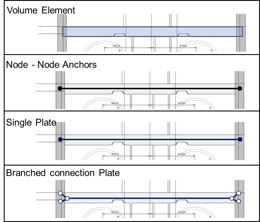
Figure 10 – Slab-wall connections The tunnel construction has been modelled with a volume loss value of 0.7% for a 300mm continuous concrete lining, considering no contribution from the grout (Table 7).
Table 7 – Properties of Tunnel Lining
Parameter Name Value Unit Elastic Modulus E E 210000 MN/m2 Axial stiffness EA/s 9900 MN/m Flexural stiffness EI/s 74.25 MNm2/m Weight W 6.9 kN/m Poisson’s ratio ν 0.2 – Construction Sequence
The construction sequence modelled in Plaxis consists of Stage numbers 1 to 25. The key stages reviewed for the performance of the diaphragm wall are shown in Table 8.
Table 8 – Key Construction Stages Modelled in Plaxis
Plaxis Stage Stage Description Stage 5 Install diaphragm wall, bored pile and plunge columns Stage 6 Install tunnels Stage 7 Excavate to roof slab blinding at level 121.925 m ATD Stage 8 Install roof slab Stage 11a Excavate to interchange level at 117.05 m ATD Stage 12 Excavate to 113.6 m ATD Stage 13 Install temp preloaded prop at level 114.5 m ATD Stage 14 Excavate to concourse blinding at level 111.30 m ATD Stage 15 Construct concourse slab Stage 16a Remove temp prop Stage 16b Install intermediate slab Stage 17 Excavate to base slab level 102.560 m ATD Stage 18 Install base slabs Stage 24c Long term condition Stage 25 Applying potential future development 75 kPa surcharge Measured Deflections
The wall deflections were monitored by inclinometers during construction and were subsequently corrected to account for systematic errors. With a ratio B/L of 0.08 (i.e. excavation width over length), the inclinometer data of Section B are considered to be representative of plane strain conditions, free of any corner effects.
Results
With construction complete, the monitoring data has enabled the performance of the FE model to be assessed. A comparison of the measured wall displacements for the key excavation stages from two inclinometers within the perimeter diaphragm wall along both Departures Road and Eastbourne Terrace against those predicted from the Undrained (A) HSS model (case e), are presented in Figure 11. As shown in the figure, the wall displacement predictions for the Eastbourne Terrace wall are generally in good correlation with the field measurements, especially in the final stages. The predicted profiles for the Departures Road wall are close to the field data at depth below the base slab level, but deviate both in shape and magnitude at higher levels.
Inclinometer data for the Departures Road diaphragm wall was only available from the start of Stage 7 and thus all the relevant deflection profiles were assumed to commence from this stage (i.e. reset to Stage 7). The inclinometer data for the Eastbourne Terrace diaphragm wall was available from the beginning of the construction.
The maximum wall deflection at the final excavation stage occurs near the excavation level, i.e. the base slab level, comprising approximately 0.1% of the excavation depth. Table 9 and Table 10 summarise the maximum deflections, bending moments and shear forces during the excavation to the base slab level (Stage 17) for the FE models and the sensitivity cases considered in this paper.
Table 9 – Deflection results, Ux, from FE models for Stage 17
FE model Diaphragm Wall Horizontal Deflection (mm) Departures Road Eastbourne Terrace Case a MC – Undrained (A) 26 30 Case b MC – Undrained (B) 21 26 Case c HS – Undrained (A) 16 26 Case d HS – Undrained (B) 16 21 Case e HSS – Undrained (A) 15 25 Case f HSS – Undrained (B) 14 19 Case g MC with 3E’ for passive side – Undrained (A) 22 26 Case h MC with 3E’ for passive side – Undrained (B) 16 22 Case i HSS – Undrained (A) with increased by a factored of 10 13 20 Case j HSS – Undrained (A) with decreased by a factored of 10 16 27 Case k HSS – Undrained (A) with Floor Connections as a single Plate 10 26 Case l HSS – Undrained (A) – Drained Conditions on Active Side 24 39 Table 10 – Maximum Moments and Shear Forces results from FE models for Stage 17
FE model Diaphragm Wall Bending Moment (kNm/m run) Diaphragm Wall Shear Force (kN/m run) Departures Road Eastbourne Terrace Departures Road Eastbourne Terrace Case a MC – Undrained (A) 1588 1791 1135 1744 Case b MC – Undrained (B) 1605 1499 975 1566 Case c HS – Undrained (A) 1320 2026 1430 2262 Case d HS – Undrained (B) 1491 1347 975 1438 Case e HSS – Undrained (A) 1308 1975 1438 2279 Case f HSS – Undrained (B) 1501 1187 917 1348 Case g MC with 3E’ for passive side – Undrained (A) 1443 2052 1270 1976 Case h MC with 3E’ for passive side – Undrained (B) 1709 1620 1014 1664 Case i HSS – Undrained (A) with increased by a factored of 10 1302 1750 1334 2048 Case j HSS – Undrained (A) with decreased by a factored of 10 1342 2065 1462 2336 Case k HSS – Undrained (A) with Floor Connections as a single Plate 1320 1983 1488 2582 Case l HSS – Undrained (A) – Drained Conditions on Active Side 1580 3003 1980 3171 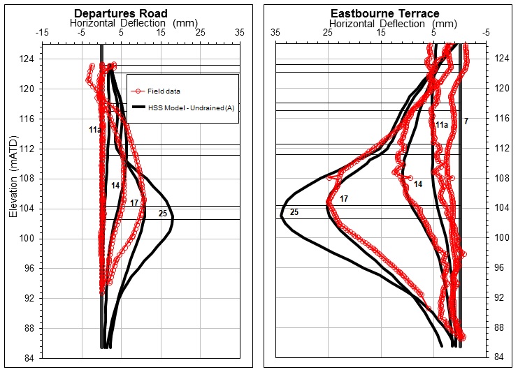
Figure 11 – Deflection profile for HSS model – Method A (case e) Effect of Drainage Condition on Active Side
Drained conditions on the active side and undrained conditions on the passive side during excavation and construction of the permanent slabs were original adopted in design in accordance with CEDS-3. The predicted wall deflection profile for this drained/undrained (case l) are presented in Figure 12 and show that the analysis over predicts the deflections by 50 to 60 %.
For all subsequent analysis cases (a) to (k) fully undrained conditions have been adopted for both the active and passive side.
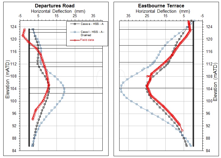
Figure 12 – Effect of drainage condition on Active Side for Stage 17 Effect of Undrained Analysis Approach (A) and (B) on MC, HS and HSS models
The performance of the three different constitutive models adopted for the deep excavation in London Clay to be assessed for both the Undrained (A) and (B) approaches are considered in cases (a) to (f). Figure 13 shows the comparison of the different FE models for Stage 17, i.e. the final excavation to the base slab level. When comparing the resulting deformations, it is clear that they all give results of similar magnitude, with maximum deflections varying between approximately 14-26 mm for the Departures Road Wall and 19-30 mm for the Eastbourne Terrace Road. This corresponds to a difference of 73 % on Departures Road Wall and 23 % on the Eastbourne Terrace Road between the maximum model deflections and the actual ones.
Figure 13 also shows that the maximum deflections for Eastbourne Terrace above the base slab, derived by the HSS (case e) and HS models (case c) with Undrained (A), match the maximum measured data at the same level.
It should be noted that the MC Model using Undrained (A) resulted in the greatest differences, over predicting by up to 73 % compared to the measured data. The HSS Model using Undrained (B) under-predicts the wall deflections below the intermediate slab level by up to 23 %.
The Undrained (A) Approach for all three constitutive models resulted in higher deflection predictions by up to 6 mm compared to the Undrained (B) Approach. In addition, the MC model predicts the largest wall deflections and the HSS the smallest as expected.
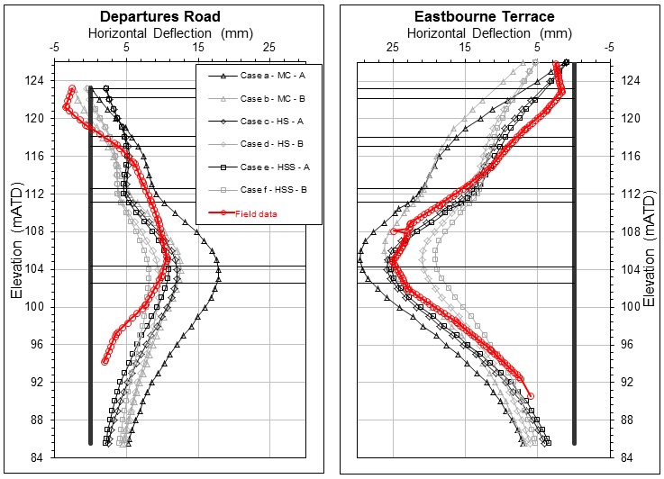
Figure 13 – Comparison of wall deflections of different FE models for Stage 17 Figure 14 and Figure 15 present the bending moments and shear forces diagrams of the different FE models for Stage 17, respectively. Very similar plots have been resulted, with HS and HSS Undrained (B) models generally yielding lower moments and shear forces, especially below the intermediate slab level. It can also be seen that the Eastbourne Terrace wall is expected to carry greater structural loads compared to the Departures Road wall.
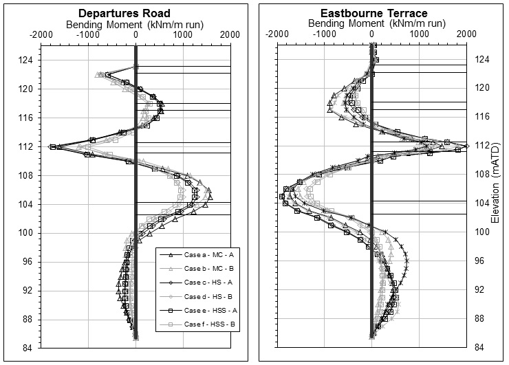
Figure 14 – Comparison of bending moments of different FE models – Stage 17 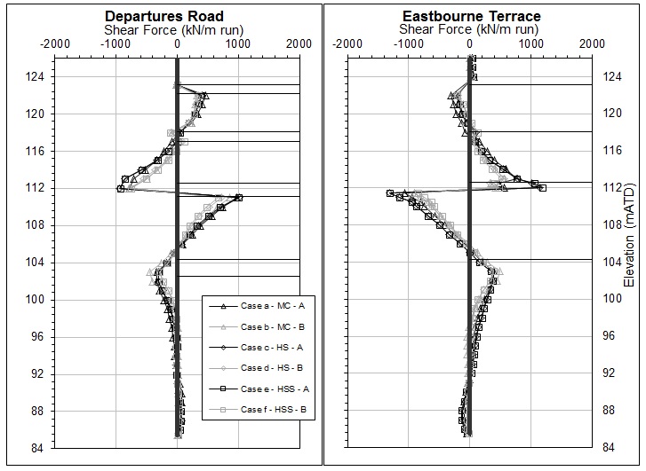
Figure 15 – Comparison of shear forces of different FE models – Stage 17 Effect of Modelling Unload-Reload stiffness on a MC model
The stress-strain relation of the MC model is linear elastic-perfectly plastic and is not able to model the unload-reload behaviour. To account for the unload-reload stiffness in the passive side, the MC models have been re-calculated by setting the Young’s Modulus to 3*E‘ in front of the diaphragm wall within the station box excavation. As expected, these analyses have yielded up to 5 mm lower deflection values compared to the original analyses with the single value E‘ for the entire London Clay (Figure 16). The resulting deflected profile for the Undrained (A) case is closer the measured data, whereas the Undrained (B) results in under-prediction of the deflections.
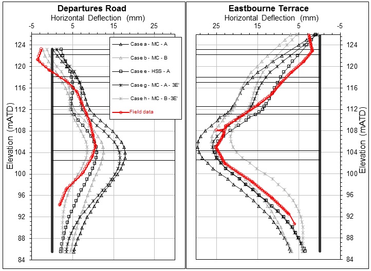
Figure 16 – Comparison of deflections between E’ and 3*E’ MC models – Stage 17 Effect of γ0.7 on HSS model
The γ0.7 to be used in the FE model needs to be carefully considered prior to any analysis and its effect on the results should be investigated. Thus, two sensitivity cases have been analysed with a γ0.7 value equal to 0.1 and 10 times the γ0.7 of the original HSS model.
The comparison of the FE models in Figure 17 reveals 20% differences between the predicted deformations, proving that the HSS model is highly dependent on the assumed γ0.7 value. It is evident that the lower the γ0.7 value gets the greater the increase of the wall deflections are. There are various empirical correlations for γ0.7[1], thus making the selection of this sensitive parameter more difficult.
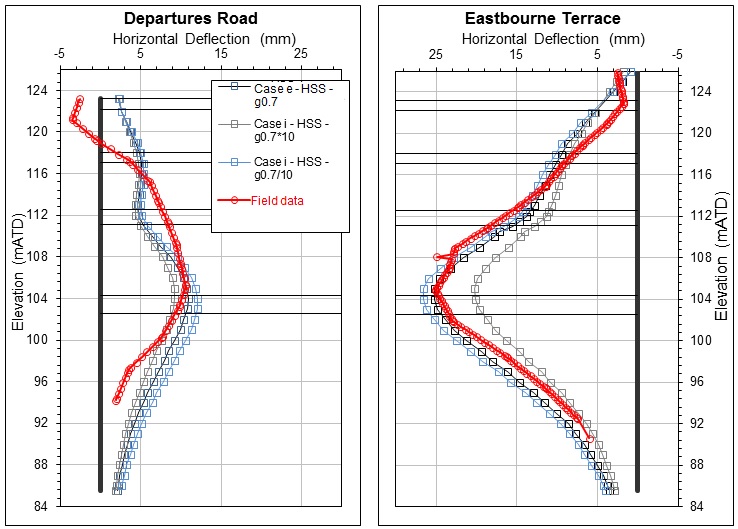
Figure 17 – Effect of γ0.7 on HSS model – Stage 17 Effect of slab-wall connection type on HSS model
A further analysis has been carried out in order to investigate the effect of the connection type, when varied from branched to single plate connection. As shown in Figure 18, this has returned steep changes, “jumps”, in bending at the slab connection levels, but marginally different diagrams for the remaining part of the wall. However, it should be noted that the difference in bending or shear with the original model was no more than 12% at any connection point, thus indicating the small effect of the parameter in the analysis.
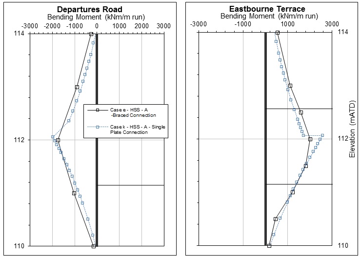
Figure 18 – Effect of slab-wall connection in bending for stage 17 Conclusion
The CEDS-3 recommended drained/undrained analysis was found to be more conservative compared to the fully undrained analysis, implying that the undrained conditions are more representative for the two year construction period of Crossrail Paddington station.
The influence of using effective and total strength parameters for these different ground constitutive models on the performance of the Paddington Station diaphragm wall has been investigated. All models compared reasonably well with the measured wall deflections, with Undrained (B) analyses showing lower deflections in all cases compared to the Undrained (A). As expected, the MC Undrained (A) and (B) analyses indicated larger deflections than the HS and HSS model predictions.
The HSS Undrained (A) analysis showed the best overall fit to the field data, both in shape and magnitude, especially for the final stages. Nevertheless, the narrow range of the predicted deflections of all models and the uncertainty involved in determining the HSS input parameters G0 and γ0.7, show that there is no advantage in using the more advanced HSS model compared to HS or MC constitutive models for the design of the diaphragm walls. This may not be the case when assessing the settlements behind the wall where the strains will vary. It should be expected that for a relatively small strain deformations, HSS model should provide the closest results to the actual value. With relatively large strains, the conventional ground models (MC) should provide acceptable accuracy.
It becomes clear that further research is required in the standardisation of the FE analysis regarding the selection of the stress analysis, the soil model and subsequently the relevant stiffness parameters to be input.
References
[1] Alpan, I. (1970). The geotechnical properties of soils. Earth Science, 6, 5–49.
[2] Benz, T. (2006). Small-Strain Stiffness of Soils and its Numerical Consequences. Ph.D . Thesis, Universität Stuttgart.
[3] Brinkgreve, R. B. (2009). Introduction to nonlinear soil behaviour. Plaxis Introductory Course. Glasgow: Plaxis B.V.
[4] Brinkgreve R., Broere W., & Waterman D., Plaxis 2D (2015). Reference and Materials Model Manual, Eds., Amsterdam, Netherlands: PLaxis BV.
[5] Brouwer, J. J. (2002). Guide to Penetration Testing. East Sussex: Lankelma.
[6] BSI (1994). BS 8002: 1994 Foundations. London: British Standards Institution.
[7] Chow, Y. C., & Tan, C. M. (2007). Design of Retaining Wall and Support Systems for Deep Basement. Kuala Lumpur: G&P Geotechnics Sdn Bhd.
[8] Crossrail. (2009). Civil Engineering Design Standard – Part 3 underground Boxes and Deep foundations Report No. CR-STD-303-3. Ver. 6.0. London.
[9] Davies, R. V., & Whittle, A. J. (2006). Nicoll Highway Collapse: Evaluation of Geotechnical Factors Affecting Design of Excavation Support System. International Conference on Deep Excavations. Singapore.
[10] Duncan, J. M., & Chang, C. Y. (1970). Nonlinear analysis of stress and strain in soils. Journal of the Soil Mechanics and Foundations Division, 1629-1653.
[11] Hardin, B. O., & Drnevich, V. P. (1972). Shear modulus and damping in soils: Design equations and curves. Journal of the Soil Mechanics and Foundations Division, 667-692.
[12] Johansson, E., & Sandeman, E. (2014). Modelling of a deep excavation in soft clay A comparison of different calculation methods to in-situ measurement. Chalmers University of Technology.
[13] Santos, J. A., & Correia, A. G. (2001). Reference threshold shear strain of soil, its application to obtain a unique strain-dependent shear modulus curve for soil. Proceedings of 15th international conference on Soil Mechanics and Geotechnical Engineering, (pp. 267-270). Istanbul.
[14] Vardanega, P. J., & Bolton, M. D. (2013). Stiffness of Clays and Silts: Normalizing Shear Modulus and Shear Strain. Journal Of Geotechnical And Geoenvironmental Engineering, 1575-1589.
-
Authors