Correlation study between in-situ auscultation and satellite interferometry for the assessment of nonlinear ground motion on Crossrail London
Document
type: Technical Paper
Author:
Javier Garcia Robles, Mike Black BSc(Hons) MSc CSci CGeol FGS, Borja Salvá Gomar, ICE Publishing
Publication
Date: 31/08/2016
-
Read the full document
Notation
InSAR (Interferometry Synthetic Aperture Radar)
PSI (Persistent Scatter Interferometry)
TS (Time Series)1 Introduction
This paper aims to provide a cross-checked overview of two different and independent techniques used to assess the state of the stability of London works conducted by Crossrail Limited over the entire city. The two techniques compared are Radar Persistent Scatter Interferometry technique carried out by Altamira Information for Crossrail Ltd, and auscultation measurements, such as precise levelling networks, robotic theodolites, hydrostatic level cell networks or tilt-meters, carried out by Crossrail Ltd and their contractors.
Both types of measurements have diverse objectives. While auscultation measurements are almost continuous data which involve a real-time assessment of the impact of the works carried out in the scene and very close surroundings in several specific chosen points in order to avoid risk or mitigate its impact, InSAR is a non-real time technique which works with discrete data and can assess vast areas using images acquired on different dates separated by days/weeks or months, allowing an insight of local and large displacement bowls during the period analysed. Thus, it can be affirmed that both techniques are complementary and add value to each other.
In view of this, a correlation study between both datasets was conducted in order to calibrate and prove the quality of the measurements, representing them in the InSAR scale of time and magnitude provided that an overlapped period existed. This study reflected the consistency and complementarity of both techniques when it comes time to monitor the impact of infrastructure construction.
All the research was conducted under the framework project of “Historical ground motion study for Crossrail London using Interferometric Synthetic Aperture Radar Persistent Scatter Interferometery”, presented in London on October 2015, whose objective was to prove InSAR as an operational technology of ground motion monitoring in civil engineering work scenarios, of which followed the subsequent framework project “X9171 Post Works Ground Surface Monitoring using Interferometric Synthetic Aperture Radar Persistent Scatter Interferometery” (ongoing).
2 InSAR measurements
Interferometric synthetic aperture radar method uses a set of SAR images to generate maps of surface deformation, although it can also be used for other purposes such as Digital Elevation Model generation. A SAR Interferogram is defined as the phase-difference between any two acquisitions. Once the impact of topography and the flat earth effect are removed, the phase component of these pairs, known as a differential interferogram, shows ground motion that occurred between both acquisitions.
The motion signal appears as phase fringes in interferograms, and the number of fringes depends on the magnitude of motion and the satellite wavelength. In the case study presented, X-band satellites were used, meaning that one fringe corresponds to ground motion of approximately 1.55 cm. Interferogram colour scale ranges cyclically from blue to red and represents values between -p and +p radians. Slight motion generates spatially separated fringes, while motion that is occurring at a more accelerated rate, produces closer fringes.
When a displacement in the interferograms is observed constantly and proportionally over time, it can be affirmed that linear motion is occurring, so ground motion is reflected with a constant trend on the Time Series. On the other hand, when the motion appears to be sudden, concentrated only in some images of the full stack, has variations in its intensity, area and/or trend (subsidence, stability and heave alternated), it can be affirmed that nonlinear motion is occurring. Nonlinear ground motion is reflected with different trends on the Time Series and may be not easily detectable.
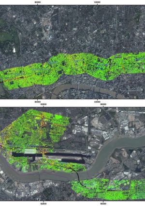
The temporal study of a sequence of interferograms allows the identification of strong nonlinear patterns. In order to illustrate this, the interferogram of Figure 1 (b), displays the phase variation associated to a deformation pattern detected over the line path between High Park and Bond Street Station. It is also notable the motion detected surrounding the TCR station.
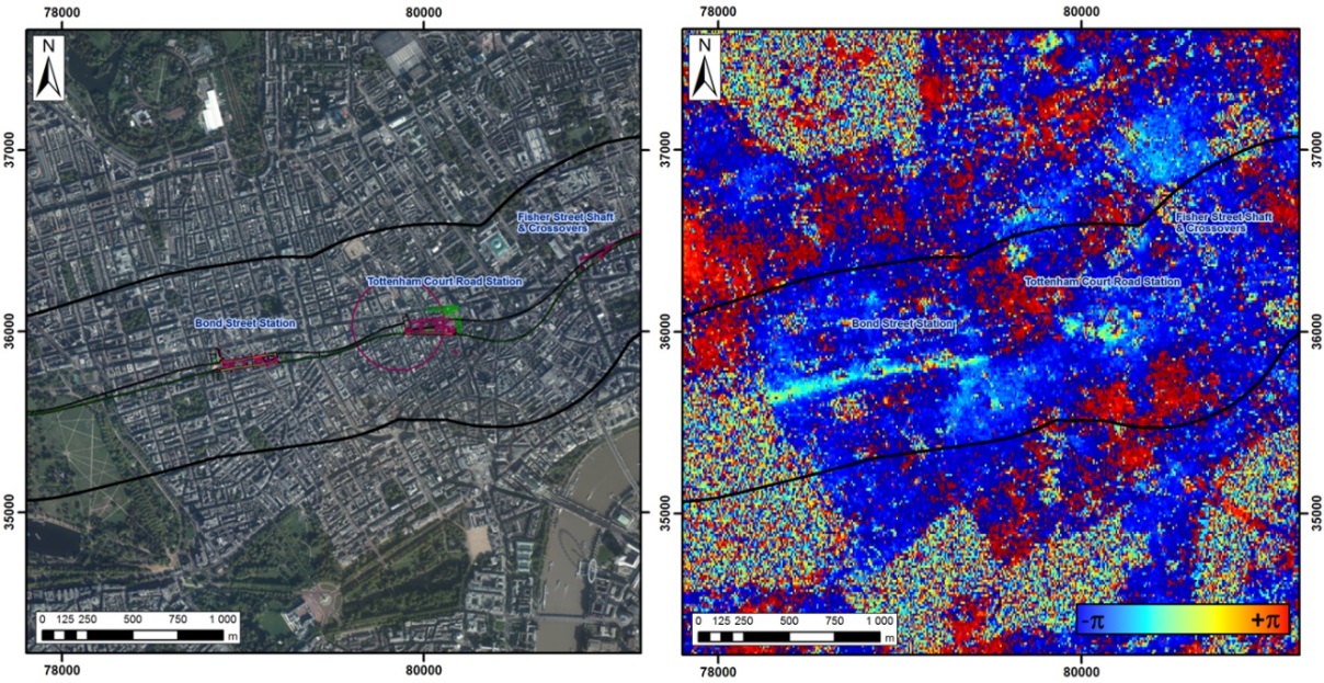
Figure 1 – (a) Aerial orthophoto between High Park and TCR with the track line and stations, (b) Overlayed differential Interferogram between dates 11/08/2012 and 10/05/2013, detecting motion over Crossrail Line. The differential interferograms are the input to the Persistent Scatter Interferometry (PSI) processing chains. As more SAR acquisitions are available the higher amount of relations (interferograms) between these acquisitions can be computed and thus the higher detail of data will be obtained.
2.1 PSI methodology approach used
Persistent Scatter Interferometry (PSI) based algorithms are the conventional tools used to detect and precisely estimate ground motion in a set of radar images within a concrete time span. Each interferogram contains different components related to different magnitudes that are potentially measurable and useful in the subsequent steps of the processing. However, there are some of the components that are not of interest in terms of ground motion, and the objective is to remove them from the original phase to allow motion detection. The latter is achieved through PSI algorithms.
Furthermore, two separated blocks of components can be set: the linear block and the nonlinear block. The linear block can be easily estimated thanks to its direct relation with a linear input model. The nonlinear block in contrast, is more complex to be estimated as has no relation to any initial model and has to be removed either using spatial and spectral filtering processes or simplified using advanced estimation atmosphere and nonlinear models. The following equation (1) shows the possible phase terms present in an interferogram.
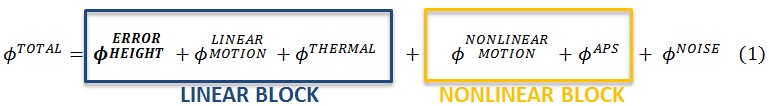
In the specific case of PSI techniques that use an initial lineal model of displacement in time as an input to isolate the nonlinear components, and always provided that slight variations from the linear trend and not strong nonlinear motion exist, PSI linear model techniques are able to retrieve the slight nonlinear motion, incorporating it to the general linear trend of the time series without carrying out the unwrapping step. This approach is shown in Figure 2.
Figure 2 – PSI method with an initial linear model approach. It can be used as well to delimitate the nonlinear areas. When the ground motion does not have linear dependence on time, for instance in the case of different trends and even strong variations, such as the alternation of periods of heave and subsidence, the linear deformation model to estimate the atmosphere is not applicable. This is because the behaviour in space and time of the atmosphere and motion has a common part in the spectral/temporal domain. A new approach, outlined in Figure 3, is therefore needed to be able to retrieve accurate measurements, irrespective of the motion being linear or nonlinear. In these cases, the linear quality fitting parameter (linear model coherence) can be a very significant parameter to delimitate areas affected by nonlinear motion.
Interferometric coherence is the most appropriate statistical indicator to check whether the studied area has nonlinear behaviour or not. There are two types of coherence indicators: the mean interferometric coherence, which is dependent on the spatial and temporal decorrelations, but not sensitive to the nonlinearity of the motion; and the lineal deformation model coherence which is dependent on how the evolution of the measurement phase is adapted to a particular deformation rate trend and is very sensitive to the nonlinearity.
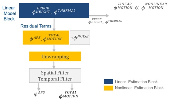
Figure 3 – PSI method with a nonlinear model approach. The mean coherence is a measure of the correlation of the phase information of two corresponding signals and varies in the range of 0 to 1. The degree of coherence can be used as a quality measure: coherence near 1 means the phase information is reliable (and the images have high degree of correlation), whereas coherence < ~ 0.3 means the images have low correlation (noisy). In this case, the phase information is probably not useful.
The lineal model deformation coherence is a quality measure which relates to the millimetric measurement model (average annual displacement rate) fit. Values between 0 and 1, where 1 indicates best fit. The fitting quality depends on the characteristics of each processing, like the number of images used, the noise level of the measurement point and the reliability of the model fitting.
In Figure 3 below, a comparison between mean interferometric coherence and linear deformation model coherence is shown. The bright points in the mean coherence values reflect points that are measurable, while bright points in the model coherence reflect points that have a good estimation of deformation with the process conducted.
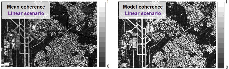
Figure 4 – Mean coherence (left) and lineal model coherence (right) in a lineal scenario of an urban area close to an airport. In the opposite case, in Figure 4, it is obvious the diminution of the coherence value in the nonlinear case of a sewerage facility which showed signs of motion. It is evident that, the mean interferometric coherence shows high coherence level in an area where the model coherence shows lower values. This behaviour of the model coherence is typical in nonlinear ground motion areas.
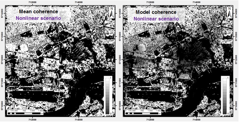
Figure 5 – Mean interferometric coherence and lineal-model coherence on a sewerage tunnelling, reflecting nonlinear motion. Some general conclusions can be extracted analysing the comparison between both coherences in the lineal and nonlinear deformation cases.
- Either linear or nonlinear motion areas present high interferometric mean coherence for the full interferometric stack (See left plots on Figure 4 and Figure 5) independently of the existing nature or motion.
- Nonlinear motion areas present low model coherence in regular lineal velocity estimation. That is why the linear approach aids in the detection and delimitation of nonlinear areas (See right plot on Figure 4).
In order to retrieve the motion and discard other contributions in the phase such as the atmosphere phase screen, the latter has to be removed leaving only the contribution of the ground motion in the interferograms. Both coherences (model and mean interferometric coherence) can be compared to delimitate the nonlinear areas. These nonlinear ground motion areas must be isolated from the atmosphere estimation in order to avoid its contribution to the APS computation. After this step, the APS is deducted using a set of reliable coherent points from the linear model of coherence. These points should be well spatially distributed in order to both estimate and interpolate accurately the atmosphere with temporal and spatial filters based on stochastic processes and image processing theory.
2.2 Area processed and data used
A final number of 38 Cosmo-SkyMed acquisitions (descending mode) were selected from the historical available dataset for this project. Dates for these images range from April 2011 to August 2013. The temporal distribution of these acquisitions is shown in Figure 6. It is important to note that each acquisition represents a measurement in time.
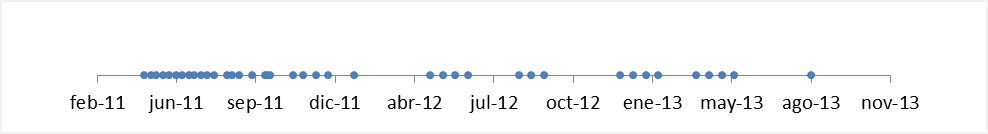
Figure 6 – Time distribution of the images. Figure 7 presents the structure of the area of interest analysed, while Table 3 gives information of the graphic schema of the highlighted areas.
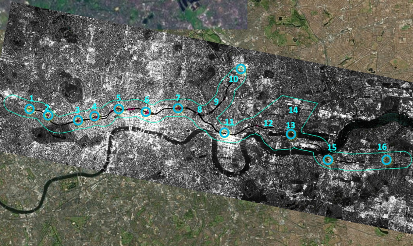
Figure 7 – Areas of interest of the study overlayed on the average amplitude radar image. Stations, shafts and portals within AOI
1 Royal Oak 9 Eleanor Street Shaft 2 Paddington Station 10 Stratford, Northern Outfall Sewer 3 Bond Street Station 11 Canary Wharf 4 Tottenham Court Road Station 12 Victoria Dock Portal, Limmo Shaft 5 Farringdon 13 Custom House 6 Liverpool Street Station 14 Beckton District and Newham 7 Whitechapel Station 15 Woolwich 8 Stepney Green Junction 16 Abbey Wood Table 3 – Detailed information of the displayed areas on Figure 7.
2.3 Results
InSAR measurement points are presented as accumulated deformation maps. The objective of those is to make clear linear and nonlinear large-scale ground motion, while also identifying areas affected by local patterns of deformation. Time Series are shown all together with the auscultation measurements in the correlation study (Section 4).
The background used is an orthophoto based in Imagery Basemap. Over this orthophoto, coloured points are presented corresponding to the measurement points that reflect a good quality signal to the satellite throughout the period of study. The colour scaling relates to the value of the accumulated displacement where green represents stability over the period of study, blue represents heave and red indicates subsidence. Figure 9 shows the colour scale used in the InSAR images presented in this section and in Correlation study section. Taking into account the dynamics of the site and the intensity of the motion patterns observed, the colour scale includes values of up to 20 mm of accumulated ground motion between April 2011 and August 2013. The stability is set at 5 mm.
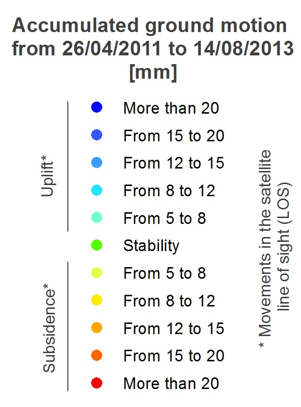
Figure 8 – Colour table used for the images of the delivery. The quantification levels are set according to the amount of displacements detected, in order to show their evolution in time. The average density of the InSAR results presented, consisted of 24,800 measurement points/km2.The results over the whole period allowed an understanding of previous vulnerable areas before the work began and seeing the evolution of pre-tunnelling works, those related with the preparation of the ground for the tunnelling works, such as dewatering and shaft creation.
As the analysis of the ground motion was being completed, it was detected that the motion present in the interferograms and the dynamics of each area were variable in time. The works were carried out on different time schedules and thus not all the sections underwent the same processes for tunnelling preparation, for instance dewatering processes, or shaft constructions. Therefore the behaviour of the subsidence was different in each timespan depending on the specific section of the AOI. The last part of the study detected the impact of the advance of the tunnel boring machine between some sections over the surface. The overall accumulated motion map is shown in Figure 9.

Figure 9 – Accumulated ground motion displacement map for London Crossrail Line. In Figure 9, the purple star marks the considered reference point, in a stable area of the processing. On this map, the path of subsidence above the Crossrail track, shafts and stations is clear. Other areas affected by dewatering and reabsorption of water show different tendencies and aspects of motion depending on the work carried out on the soil.
Two areas have been selected as they shown the evolution in time of the motion very clearly. The subsidence track of Bond Street, which follows the northeast-southwest direction, is detected between February and May 2013. The commented subsidence is located between Regent St. and Berkley St. following Conduit St.
Victoria Dock Portal and Limmo Shaft are enclosed within the areas with more motion of the study (Figure 11). Motion is detected within Leamouth Peninsula, Limmo Peninsula Ecological Park, Wharfside Rd, East India Dock Rd, A13 Newham Way, Lower Lea Crossing, Barking Rd and surrounds. Stability in the area lasted until January 2012, then from this date until April 2012 slight subsidence is detected in the whole area which continues increasing until September 2012. Between September 2012 and December 2012 heave is detected thus reducing the extent of the accumulated subsidence. In the following months no significant motion is detected, until April 2013, when once again subsidence is detected, which increases between May and August 2013.
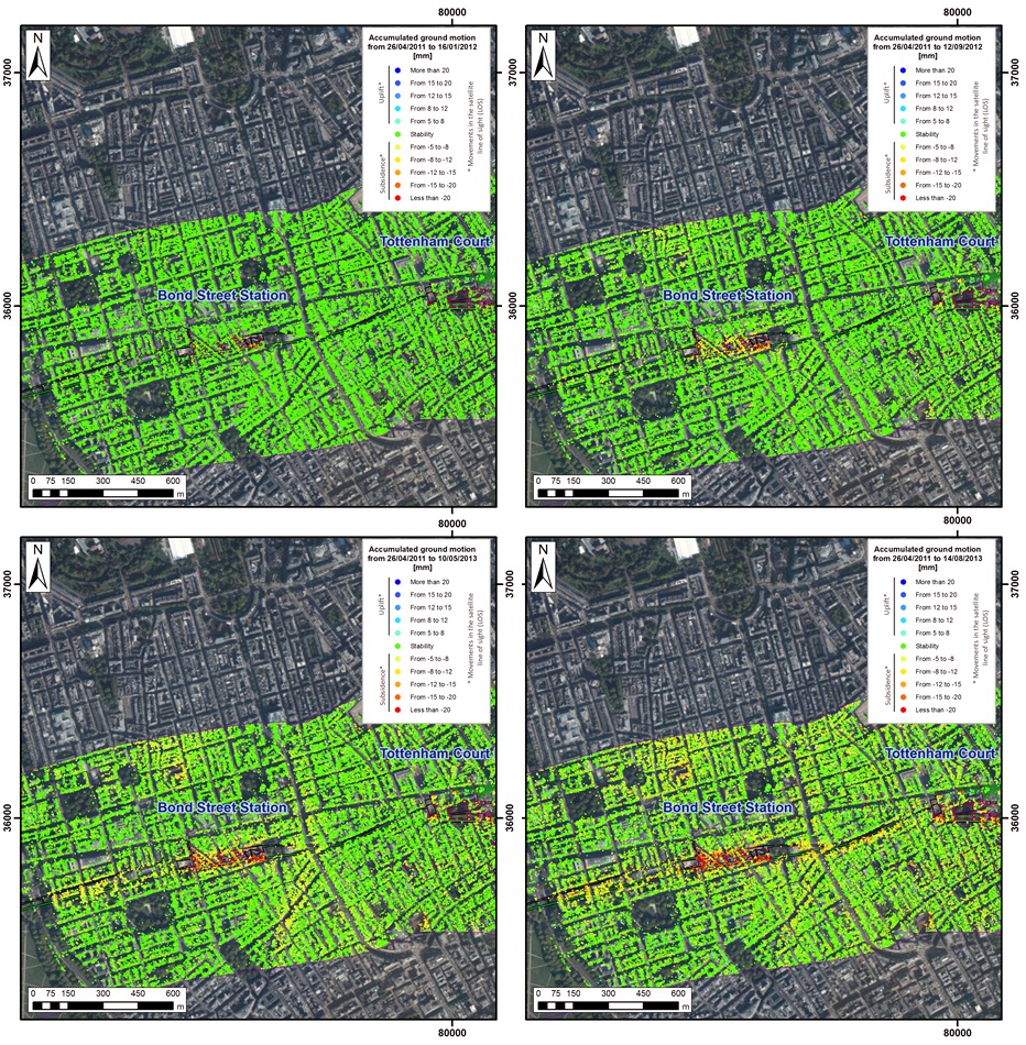
Figure 10 – Setting temporal reference on April 2011, evolution of accumulated motion from January 2012 to August 2013 in Bond Street Station and surrounds. 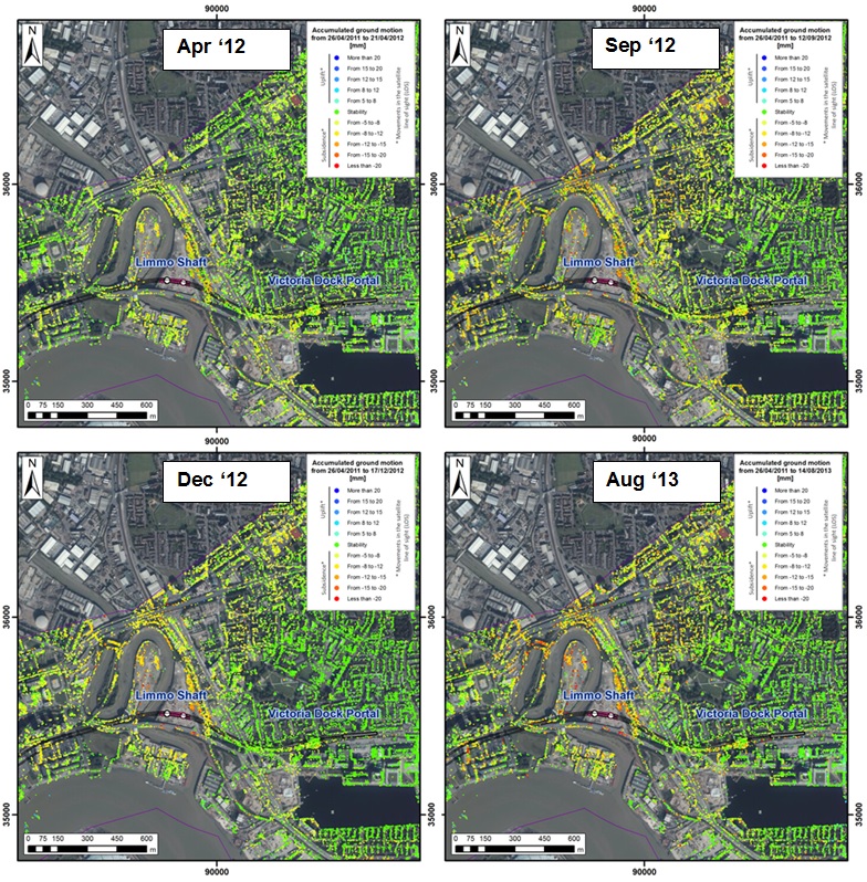
Figure 11 – Setting temporal reference on April 2011, evolution of accumulated motion from April 2012 to August 2013 on Limmo Shaft and Victoria Dock Portal. 3 Auscultation measurements
Monitoring has been undertaken on the Crossrail project for a number of core purposes. The principle objectives of the monitoring were as follows:
- Construction process control –to inform decisions made as an integral part of construction activities;
- Design verification – to validate assumptions or predictions made during the design.
- Third party asset protection – to provide data, which may be used in connection with contingency plans, to protect existing third party assets or their operation;
- Risk and liability allocation – to provide evidence to determine which works caused which effect and thereby determine which party may be accountable for the consequences of that effect;
A number of different techniques and instrumentation were employed for monitoring the progress of the works in line with the above criteria. Across the central tunneled section of the route (i.e. the area that coincides with the InSAR study), approximately 75,000 instruments or monitoring points were installed. These consisted primarily of ground surface or building movement points in the form of studs or reflective prisms/targets for precise levelling or automatic total stations. Building movement and, in particular, differential movements within buildings was also monitored using hydraulic levelling cells (HLCs). Aside from providing valuable information for asset protection purposes, HLCs proved to be particularly useful in controlling the effects of compensation grouting, a technique used to mitigate the effects of tunnelling induced ground movement.
Additional instrumentation such as crack meters, inclinometers and electrolevels were used to monitor specific buildings or structures. Whilst providing important information at a local level, these were less useful for correlation purposes with the InSAR study, which relied primarily on precise levelling and total station data.
Given the location of the Crossrail works and the sensitivity of the surrounding urban environment, the frequency of readings for conventional monitoring such as that described above, was scheduled to allow rapid (in some cases near real-time) provision of information during the active construction works. The resulting data was reported by the respective project teams every shift, to ensure that trends in movement were identified early and any necessary actions implemented to allow the safe continuation of work. The precise levelling and total station monitoring had a specified accuracy of +/- 1mm.
The frequency of monitoring reduced following the successful completion of each element of construction, until the rate of movement was demonstrated to have effectively ceased. This equated to a rate of 2mm/year, demonstrated by 4 consecutive readings over a 12 month period. It was considered that InSAR could potentially substitute for this phase of monitoring, with the benefit of providing more widespread data coverage than conventional monitoring alone.
4 Correlation study
Several time series plots have been selected from the correlation study, carried out between levelling and Total Station Crossrail data and InSAR data for the overlap periods. These correlation Time Series present a comparison of the data of both techniques, complement the information and validate one of the techniques with the other. In most of the cases the amount of discrete data allows only a concrete time-span of overlap between both datasets.
InSAR data is able to assess the motion pattern before some of the in-situ measurements were being carried out; in contrast, auscultation has more continuous measurements and could establish better the behaviour of the evolution of motion in real time. Crossrail levelling data is plotted in black marks, while InSAR data from Altamira Information study is plotted in coloured dots.
On Figure 12 correlation TS are shown in the proximity of the junction of N. Audley St. and Lees Pl. The main event worth noting is the strong increase of motion of 5-6 mm that occurred in March 2013. In some cases calibration may show a constant offset between InSAR data and Crossrail data derived from a variable reference of calibration, as occurred in the lower correlation plot shown.
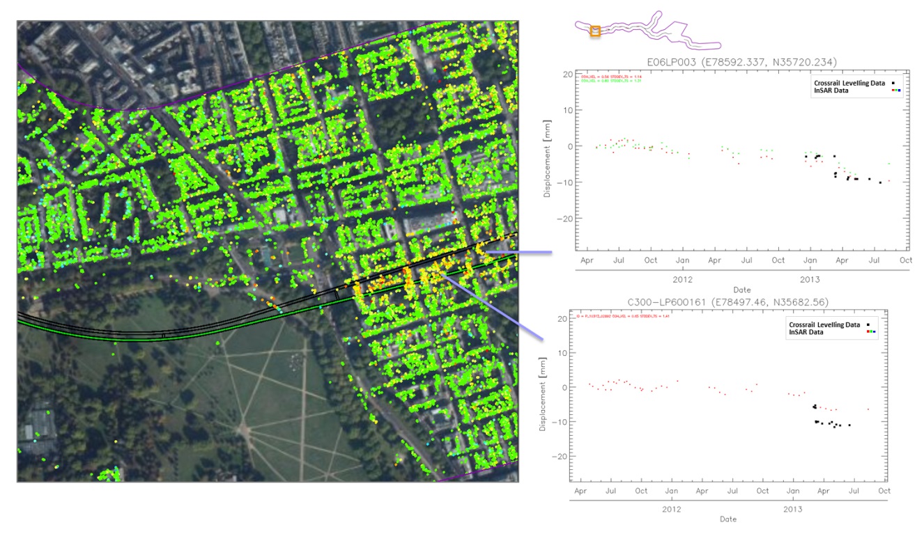
Figure 12 – Selected TS from the correlation study of both techniques in the proximity of the junction of N. Audley St. and Lees Pl. The correlation plot for New Bond St. junction with Blenheim St. (Upper plot in Figure 13), shows strong subsidence between May and June 2012, following this, heave is detected and continues until January 2013. Linear subsidence is then detected during the rest of the period between January 2013 and August 2013. In the correlation plot between Oxford St. and Tenterden St shown in Figure 14, a larger overlap is achieved. Motion is detected from February 2012 until September 2012. Following this, a slight trend of subsidence is detected.
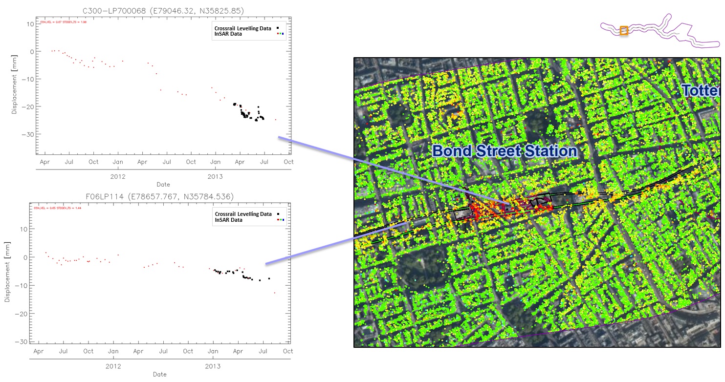
Figure 13 – Selected TS from the correlation study of both techniques in the western part of Bond Street station. 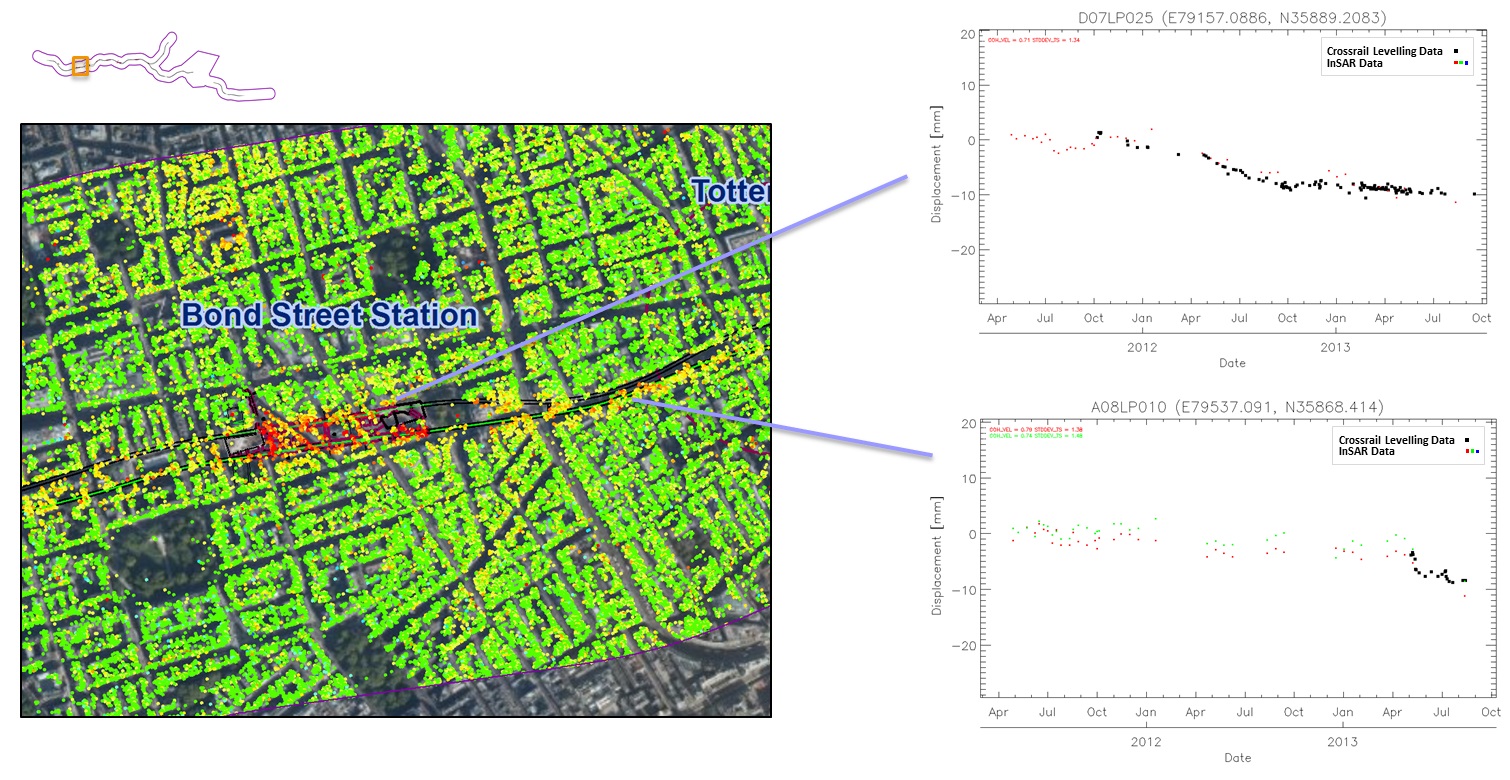
Figure 14 – Selected TS from the correlation study of both techniques in the eastern part of Bond Street station. Two correlation plots from the area have been selected to show the comparison between both datasets. The top plot of Figure 15 shows nonlinear motion detected in the north-eastern corner of Soho Square. Both datasets coincide in the overlap period detecting subsidence and also in the sudden heave behaviour occurring shortly before April 2013 which lasted for a period of less than one month. The lower TS chart shows a subsidence reaching 8 mm in the vicinity of Manette St.
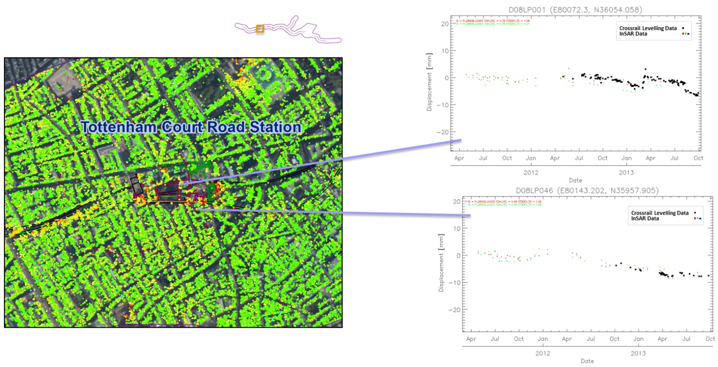
Figure 15 – Selected TS from the correlation study of both techniques in the eastern part of TCR station. Two correlation plots have been selected in a building on the junction of Brady St and Durward St. Regarding, see Figure 16. Levelling time series show an increase of the subsidence of 10 mm on June 2013. Although the upper and lower TS charts have a different evolution in time, they both reach 10 mm of accumulated subsidence. Whilst in the western part of the building the motion started in September 2012 and was more constant, in the Brady St part it was more abrupt and lasted only during the month of June 2013.
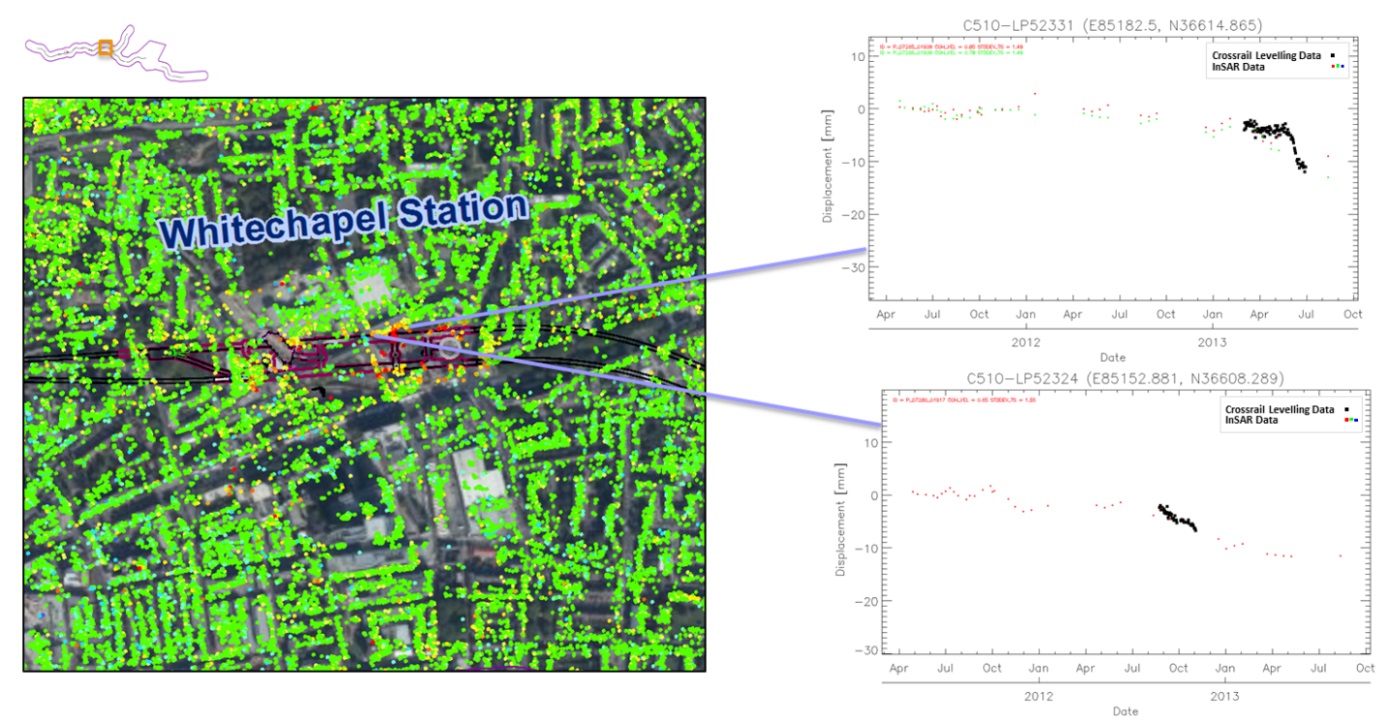
Figure 16 – Selected TS from the correlation study of both techniques in Whitechapel Station. According to the correlation TS in Figure 17, both data sets coincide in the temporal evolution of the nonlinear motion. Some of the motion shows an increase in the last period of study, which according to the levelling data reaches 10 mm of subsidence in some areas. The top graph shows data related to the bridge that crosses River Lea. The lower graph shows data related to A12 borders.
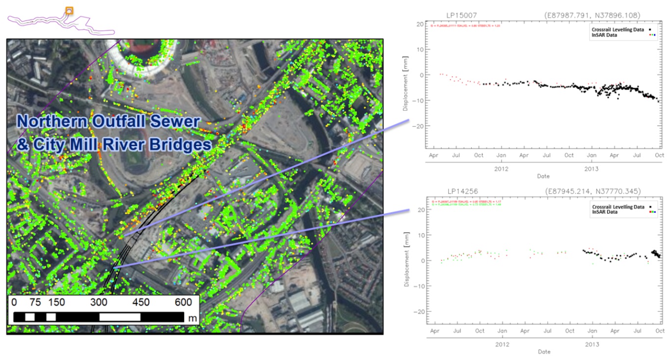
Figure 17 – Selected TS from the correlation study of both techniques on Northern Outfall Sewer & City Mill River Bridges. In the example on Figure 18, the upper TS of the correlation study nearly match. The time series retrieves the nonlinear, slight subsidence of the area which reaches an accumulated total of 10 mm.
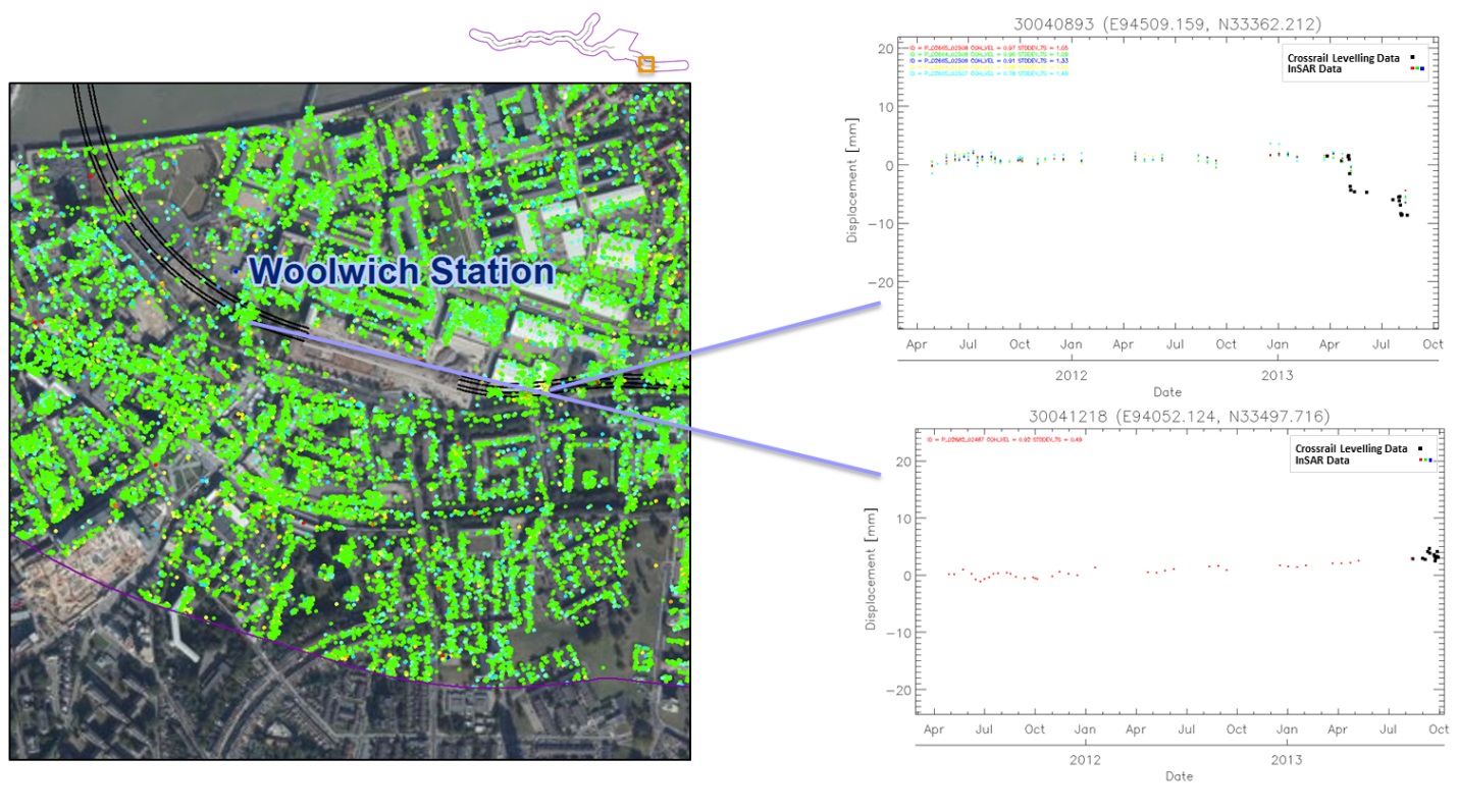
Figure 18 – Selected TS from the correlation study of both techniques on Woolwich Station. 5 Conclusions
The combination of both techniques aims to contribute to the ground monitoring of motion in tunnelling construction in several stages. This includes going from the historical motion affecting the area before the beginning of the work phase, going through the assessment of soil preparation before tunnel construction such as dewatering processes and following that, the related collateral effect of recharge of the aquifers, such as the detection of the motion caused by the advance of the tunnel boring machine and the subsequent subsidence during the settlement period. When strong and rapid motion is expected, it is essential to follow a sufficient satellite acquisition rate sampling in order to retrieve all the possible events.
It is obvious that combining SAR technique with in-situ measurement enhances the whole survey, as both techniques would be complementary and would perform a cross-validation of each other and aids in the calibration of both data to a specific temporal reference. The correlation study conducted confirmed the most part of the nonlinear events detected.
It is very important to have a real-time assessment with auscultation while the works are being carried out, since Interferometry can’t provide real time flux of data the way in-situ network measurements does. However, once the works have been completed, InSAR could gradually substitute in-situ measurements, when less motion is expected and the risk of sudden critical events is reduced; thus providing a more cost-effective option.
By retaining a network of conventional monitoring points, it is also possible to investigate any areas where ongoing long-term movement may be observed by InSAR and verify those observations. InSAR also provides wider areal coverage and as such encompasses those activities that may have a regional influence, such as dewatering settlement. Finally, providing an adequate temporal distribution of satellite sampling, will also increase the chances of observing any seasonal effects on ground movement.
References
[1] Garcia-Robles, J., Mora, O., Salvá, B., Innovative InSAR approach to tackle strong nonlinear time lapse Ground Motion. Ninth International Symposium on Field Measurements in Geomechanics (FMGM 2015), Sydney, Australia, 9-11 September 2015.
[2] Blanco-Sánchez, P., Mallorquí, J. J., Duque, S., and Monells, D. (2008). The Coherent Pixels Technique (CPT): An Advanced DInSAR Technique for Nonlinear Deformation Monitoring. Pure and Applied Geophysics, 165 (6), 1167-1193.
[3] Thierry, P., Deverly, F., Reppelin, M., Simonetto, E., Lembezat, C., Arnaud, A., Raucoules, D., Closset, L., King, C. Survey of linear subsidence in an urban area using a 3D geological model and satellite Differential InSAR. Géoline 2005, Lyon, France, 23-25 May 2005.
[4] Arnaud, A., Adam, N., Hanssen, R., Inglada, J., Duro, J., Closa & J., Eineder, M. ASAR ERS interferometric phase continuity. International Geoscience and Remote Sensing Symposium, Toulouse, France, 21-25 July 2003.
[5] Mora, O., Mallorqui, J., and Broquetas, A. (2003). Linear and nonlinear terrain deformation maps from a reduced set of interferometric SAR images. IEEE Transactions on Geoscience and Remote Sensing, 41 (10), 2243-2253.
[6] Berardino, P., Fornaro, G., Lanari, R., and Sansosti, E. (2002). A new algorithm for surface deformation monitoring based on small baseline differential SAR interferograms. IEEE Transactions on Geoscience and Remote Sensing, 40 (11), 2375-2383.
[7] Ferretti, A., Prati, C., & Rocca, F., Permanent scatterers in SAR interferometry. IEEE Trans. Geosci. Remote Sensing, vol. 38: pp. 2202–2212, September 2000.
[8] Usai, S. The use of man-made features for long time scale InSAR. International Geoscience and Remote Sensing Symposium, pp. 1542–1544, 3-8 August 1997.
[9] Zebker, H. A. and Rosen P., Atmospheric artefacts in interferometric synthetic aperture radar surface deformation and topographic maps. J.Geophys. Res.: Solid Earth, vol. 102, pp. 7547–7563, 1997.
-
Authors


Mike Black BSc(Hons) MSc CSci CGeol FGS - Crossrail Ltd
Mike is the Head of Geotechnics within Crossrail’s Chief Engineer’s Group. Mike’s role is to provide technical and professional leadership for all geotechnical aspects for the tunnelling and civil engineering sub-surface infrastructure work. He has been on the Crossrail Project since 1993 and has been involved in all stages of development of Crossrail from feasibility design, through the Parliamentary Bill process, ground investigations, civil design and construction. Prior to joining Crossrail, Mike worked in the oil and gas industry in the North Sea, the Channel Tunnel, the A27 Brighton & Hove Bypass and the Jubilee Line Extension.
https://www.linkedin.com/in/mike-black-4aa9b81b?trk=hp-identity-name