Performance benefits associated with elevated temperature set points and increased error deadbands for room temperature controllers
Document
type: Technical Paper
Author:
Harry Morgan MEng Eng Tech MIMechE MPWI, Wing Fung PhD MSc BSc(Eng) CEng MCIBSE, ICE Publishing
Publication
Date: 09/07/2018
-
Read the full document
1. Introduction
Crossrail are building eight new underground stations in the central area of London and it is estimated that 30% of annual energy usage for MEP services to keep those stations running will be for heating, ventilation and air conditioning (HVAC). Saving as much of this energy as possible will be beneficial in reducing costs for Crossrail. This paper will go over a temperature control regime that Crossrail has implemented to ensure that its stations will have increased efficiency with its HVAC systems in station rooms with more effective temperature controllers compared to traditional London Underground (LU) stations.
Cooling systems are provided at Crossrail stations for staff accommodations and for railway equipment. One of the key control components of the cooling system is the room temperature controller. The controller can be in the form of a simple bimetallic analogue device or microprocessor based BMS (building management system) outstation. To optimise the performance of the cooling system, it is important that an appropriate setting be made on the preferred temperature setting and the corresponding error deadband. A deadband (sometimes called a neutral zone or dead zone) for a temperature controller is an interval or band where no action occurs (the system is ‘dead’ – i.e. the output is zero). It is possible to set an error deadband around the set point to ensure that control action is only taken when the controlled variable moves outside the deadband[1]. In Crossrail, the following enhancement initiatives in room temperature control were implemented:
- Increase the set point temperature of equipment plant rooms in consideration to the improved temperature tolerance of modern day’s electronics. This should cut down the cooling load without compromising on the performance of the equipment.
- Increase the error deadband to prevent undue cycling of the chiller plant (in the case of direct expansion or variable refrigerant flow cooling system). It is not uncommon for premature failure of cooling plant because of excessive cut in and cut out of compressors arising from close temperature control.
The purpose of this paper is to analyse performance benefits of increasing error deadband of the temperature and examine the pros and cons of the two control approaches. It is recognised that adjusting the error deadband is sometimes limited by the default controller settings and is not possible hence both control options are complementary to each other. The paper begins with a description of the background information on control engineering. This paper will then outline the procedure and results of simulation work to confirm that the relaxation of room temperature control will lead to significant energy saving and enhancement of the operation of the cooling plant. The operation and creation of the simulation and the theory behind how it works will be discussed. The results of the model which compare the set point temperatures and error deadbands of two rooms used in LU stations to the same two rooms used in Crossrail stations will be shown and discussed.
An energy savings calculation will occur afterwards to determine whether energy will be saved by having a larger error deadband in the temperature controller.
2. Background
2.1 Control Engineering
Systems can be thought of as a group of interacting components around which an imaginary boundary may be drawn in order that only the inputs to the system and the corresponding outputs are considered[2].A control system simply has an output being controlled to provide a desired response with a desired performance, given a specified input. In this paper temperature controllers will be discussed.
Temperature Controllers
Temperature controllers are needed in any situation requiring a stable temperature. This can be in a situation where an object is required to be heated, cooled or both to remain at the target temperature i.e. the set point temperature, regardless of the changing environment around it or what is in the room[3].
There are two types of temperature control algorithms; open-loop and closed-loop. In an open-loop system an input is chosen, usually on the basis of experience, to give the desired process output. For temperature controllers, this would apply to continuous heating and cooling with no regard for the actual temperature output, thus having no feedback to control the process directly. The controller element simply decides what action to take in view of an input. The actuator responds to the input from the controller and initiates action to change the controlled variable to the desired value. However, closed-loop systems take a measurement of the output and feed this signal back for comparison with the desired response. This is known as a negative feedback control system because the feedback is subtracted from the input and the difference is used as the controller input[4]. Figure 1 shows the typical block diagram of a closed-loop system. In Crossrail, closed-loop temperature controllers are used for cooling systems and can be thought of as thermostats. This is because closed-loop systems have a greater accuracy and are less sensitive to disturbances.
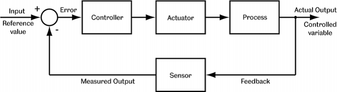
Figure 1 – Closed Loop Control System[5]
An efficient temperature controller will be able to provide just the right temperature and environmental conditions while using the minimum amount of energy from the HVAC system. Heating and cooling should not operate at the same time if an efficient HVAC system is required. However, when trying to ensure a room is maintained at a constant set point temperature, this will likely mean that both will sometimes be required. Temperature controllers could be set to enable a gap between when heating and cooling is required to reduce regular fluctuations in temperature.
This gap is known as the error deadband and can be seen in Figure 2. It can be seen that the heater has been switched on four times in this instance, however, if the error deadband was larger, there would be less fluctuations but the temperature would deviate either side of the set point more. An error deadband eliminates having both heating and cooling systems operating simultaneously and wasting energy[6]. In most railway applications, mismatch of estimated and actual cooling requirements has led to premature failure because of excessive on-off cycling.
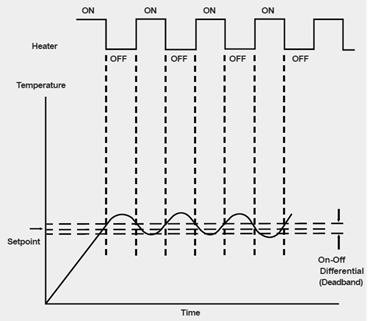
Figure 2 – On/Off Temperature Control [3]
In Crossrail, there are three types of temperature controllers in use which are shown in Table 1. It can be seen that none of the HVAC units have the ability to adjust both the set point temperature and the error deadband whilst in operation.
Table 1 – Error Deadband and Set Point on-field adjustment capabilities of three different types of Temperature Controllers used on Crossrail stations
HVAC Unit Type of Temperature Controller Set point adjustment by user On-field error Deadband Adjustment CCU (Comfort Cooling Unit) Microprocessor base Controller No Yes Fan Coil BMS based Building Management System based temperature controller No Yes Fan Coil standalone Standalone electronic temperature controller Yes No DX Digital or Variable Refrigerant Flow Units Standalone electronic temperature controller Yes, but within control range No Air Handling Unit Building Management System based temperature controller No Yes 2.2. Heating, Ventilation and Air Conditioning
Signalling Equipment Room
Across the LU network and the new Crossrail stations, in each station there will be a signalling equipment room (SER). In this study, SER is used to represent the plant room cooling requirements. Each SER are different sizes and orientations depending upon the station they’re in and each will have a different internal heating load which increases the room temperature. A SER is dedicated to containing particular signaling electrical equipment. The purpose of the room is to be a secure, environment controlled location for safe and reliable operations and maintenance. Designers and maintainers of the room are required to have a deep understanding of the complex installation, operation, maintenance and reliability of the critical systems equipment[7].
Air conditioning is regularly needed in the SER, since the electrical apparatus gives off a lot of heat but the temperature must not rise beyond the tolerance of the equipment. In the past for LU, the temperature within the rooms is set to a set point temperature in order for the equipment to not approach its maximum tolerance[8]. Electronic circuitry traditionally has operated best and most reliably at lower temperatures with higher operating temperatures decreasing the service life of the particular device so any temperature sensitive materials used in a device would degrade and wear out more quickly. However, with today’s more complex and smaller device dimensions, following the result of the development of technology in recent years, has resulted in higher heat density and elevated safe operating temperatures for electrical equipment[9].
Additionally, when temperatures fluctuate more regularly, device interconnections and other components are more at risk to fail from fatigue from expansion and contraction due to thermal stresses and fail at a faster rate than equipment whose temperature does not change as much[9].Therefore, it’s critical to minimize the temperature fluctuations by designing efficient ways of carrying away their generated heat. To address this, modern railway control equipment, are now designed to work under wider operational conditions. Crossrail has suggested that temperature controllers, for MEP rooms, accept a wider range of room temperatures. Furthermore, the number of cooling hours for MEP plant rooms should be reduced and the overall energy use for HVAC in a particular station can be reduced through the implementation of the enhancement initiative[9].
Station Supervisor’s Office
All LU stations and new Crossrail stations will have a station supervisor’s office (SSO). Similarly to the SER, each of the offices will be a different size and have a different internal heating load. The office’s purpose is to be used by the station supervisor to deliver excellent customer service by ensuring the safe and efficient operation of the station. The developments made for the temperature control of the SER with regards to enabling a wider range of room temperatures cannot be the same for the SSO. There will always be someone present in the room while the station is open and having the temperature of the room fluctuating between for instance 17°C and 27°C instead of being fixed at 22°C is not ideal for the supervisor as it’s likely that it’ll cause discomfort, despite the potential energy saving.
2.3 Simulink Blocks
In order to understand whether Crossrail station rooms will save more energy compared to traditional LU station rooms which have smaller temperature error deadbands, a dynamic model was created on the computer program; MATLAB. To create this dynamic model an additional software package, Simulink was used and the blocks used during modelling are shown in Table 2 with a small description of what each does.
Table 2 – Simulink diagrammatic Blocks with descriptions[10]
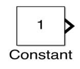
The constant block generates a real or complex constant value. In this instance it is 1, however during this project it is often used as a temperature i.e. 25°C. 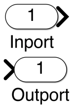
The inport and outport blocks are the links from the outside of a sub-system to the inside of a sub-system. 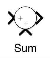
The sum block performs addition or subtraction on its inputs depending on the signs which are written on it. In this instance, both inputs would be added together. 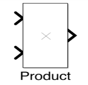
The product block is able to multiply the two inputs it has together to produce its output. 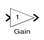
The gain block’s purpose is to multiply its input by a constant value which is whatever is set as the value for the gain. 
This block allows its output to switch between two values. When the relay is on, it will remain until the input drops below the value of the switch off parameter. When the relay is off, it remains off until the input exceeds the value of the switch on parameter. The block is able to accept one input and produces one output. 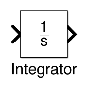
The integrator block integrated its input signal with respect to time to produce the output. 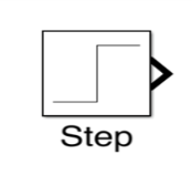
The step block provides a step between two definable levels at a specified time. For instance, if the simulation is less than the step time parameter value, the output will remain as the initial value. However, when the simulation time is greater than the step time, the output becomes the final parameter value. 
The sine wave block outputs a sinusoidal waveform. This can be used to model temperature which is varying up and down with time. How quickly this fluctuates and by much can be specified. 
The floating scope block is able to display time domain signals with respect to the time of the simulation. For instance it would be able to visualise the output of the sine wave block if a simulation was conducted. 3. Methodology
3.1. MATLAB and Simulink
MATlab is a numerical computing environment and a proprietary programming language developed by MathWorks. The program enables plotting of functions and data and with an additional software package, Simulink that allows graphical simulations and model-based designs for dynamic systems. Simulink’s primary interface is a graphical block diagramming tool and a customizable set of block libraries. Simulink is widely used in automatic control and after a free trial account was enabled for use for this project, it was chosen to be sufficient for what was available. A tutorial was found on the MathWorks website, which shows how to model a dynamic system using Simulink® software[11]. The model is of a house heating system that includes a heater (plant), thermostat (controller), and room (environment). This model has been adapted to be simulated as a Crossrail station room system which also includes a cooling unit with its own thermostat.
3.2. Procedure
Overall Modelling Goals
- Observe how changing the error deadband of the thermostat, which will be acting as the controller in this scenario, will alter the amount cycling which occurs with the cooling unit.
- Compare the differences in temperature response of a SER and a SSO.
Process Steps
- Determine the mathematical equations required to be used in creating the model.
- Collect data for model parameters to be used.
- Create the different sub-systems of the modelled system for the station room on Simulink and validate each sub-system so that it is able to function correctly during simulation.
- Conduct a parametric study to consider the effect parameters will have on room.
- Compare the differences of two rooms when the error deadband of the thermostat is changed by relating them to the set point temperatures and limits for LU[8] and Crossrail station rooms[12].
- Calculate the energy savings made by implementing larger temperature error deadbands in Crossrail station rooms compared to the traditional LU stations.
4. Modelling
4.1. Equations
This section details the equations that are required to be used with the heating unit in this model. The equations used for the cooling unit are not shown as they are similar in principle to these equations, however, rather than Qgain meaning heat gained by the heating unit, it would be cool gained by the cooling unit. See Table 3 for the descriptions of the parameters.
Rate of Heat Gain Equation
The thermal energy gain to the room is by convection of heated air from the heater. Heat gain for a mass of air in the heater is:

(1)
A fan takes room air, and passes it through the heater and back to the room. The rate of thermal energy gain from the heater is:

(2)
Since the mass of air per unit time from the heater is constant, the equation can be simplified to:

(3)
Rate of Heat Loss Equation
Thermal energy loss from the room is given by conduction through the walls, subtracted by the internal equipment heating load. In the case of the cooler operating, these would be reversed.

(4)
The rate of thermal energy loss is:
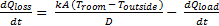
(5)
Replacing kA/D with the thermal resistance (R) means that Equation 5 simplifies to Equation 6:
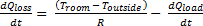
(6)
Changing the Room Temperature Equation
By defining the rate of temperature change in the room by subtracting the rate of heat loss from the rate of heat gain produces Equation 7:
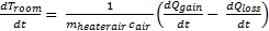
(7)
4.2. Data Collection
The values in table 3 below were used for the model[11]. All of these were kept constant throughout the modelling and analysis except k and Theater which are examined later to see what correct values would be appropriate to a station room. For this project, the most important aspect is the differences between the temperature responses whilst using different error deadbands for the thermostat with the exact temperature output being less important as there are a range of different station rooms with different sizes, resistances and internal equipment loads across the network.
Table 3 – Data used for Model
Equation Variable or Coefficient Description Units Awall Area of wall, Awall= 50 m² Dwall Depth of wall, Dwall= 0.5 m Qloss Thermal energy lost J Qgain Thermal energy gained J Qload Internal equipment load J dQ/dt Rate of thermal energy transferred J/hr K Thermal conductivity; property of a material to conduct heat transfer J/m·hr·°C R Thermal resistivity; property of a material to resist heat transfer, r = 1/k m·hr·°C/J R Thermal resistance, R = D/kA hr·°C /J U Thermal transmittance, U J/hr·m²·°C mroom Mass of air in the room, mroom= 1470 kg mheater Mass of air in the heater kg mcooler Mass of air in the cooler kg dm/dt Rate of air mass passing through the heater or cooler kg/hr Mheaterair Constant rate of air mass passing through the heater, Mheaterair= 3600 kg/hr Mcoolerair Constant rate of air mass passing through the cooler, Mcoolerair= 3600 kg/hr cair Specific heat capacity, cair= 1005.4 J/kg·°C Theater Constant air temperature from heater °C Tcooler Constant air temperature from cooler °C TroomIC Initial air temperature, TroomIC= 20 °C Troom Air temperature of room °C 4.3. Model Creation and Validation
This section goes through the creation of each of the sub-systems within the system and their validation with an explanation of the overall station room system itself.
Cooler Thermostat Sub-System
Both heater and cooler thermostats were modelled without using system equations. The thermostat for the cooling unit can be seen in Figure 3 which has a function of being able to model the operation of a thermostat that can determine whether the cooling system is on (1) or off (0). When the room temperature is above the set temperature, the control signal equals 1 to cool the room and when the room temperature is below the set temperature, the control signal equals 0 and the cooler will be switched off. This can be seen in Figure 3 with the sum block as the set room temperature has been subtracted from the room temperature to assess this. There is an error deadband attached to the thermostat which enables there to be a value either side of the set point temperature. If the control signal equals 1 then the room temperature must decrease by the error deadband’s value below the set point temperature before turning off and the thermostat changes to 0. This is done by the relay block.
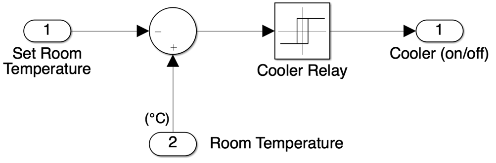
Figure 3 – Cooling Unit Thermostat Sub-system
A constant block was added to the set room temperature input for it to be 25°C.To ensure that the cooling unit thermostat sub-system would operate correctly, it was validated. This was done by thinking about its expected behaviour. When the room temperature drops below the selected set point temperature (25°C) by a selected error deadband (2°C), the thermostat output is 0. When the room temperature moves above 25°C by 2°C, the thermostat output is 1. The steps below were taken to assess whether the thermostat operates as expected. See Figure 4 to see the outside of the Thermostat sub-system with the components added to simulate it.
- A sine wave block was added to the room temperature input to represent the changing room temperature to ensure there is a variation above and below the set point temperature.
- The stop time of the simulation was set to 10 seconds and the model was run with the floating scope recording the results.
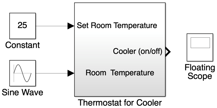
Figure 4 – Thermostat Sub-System prepared for Validation
Initially the relay was off, and the room temperature was below the set room temperature. When the room temperature increases above the set point temperature, the relay does not initially switch on until the room temperature increases to 27°C. Therefore in reality this would have signified to the cooling unit to turn on the cooler and it would have cooled the room down to 23°C. This simulation has validated the expected behaviour of the thermostat.
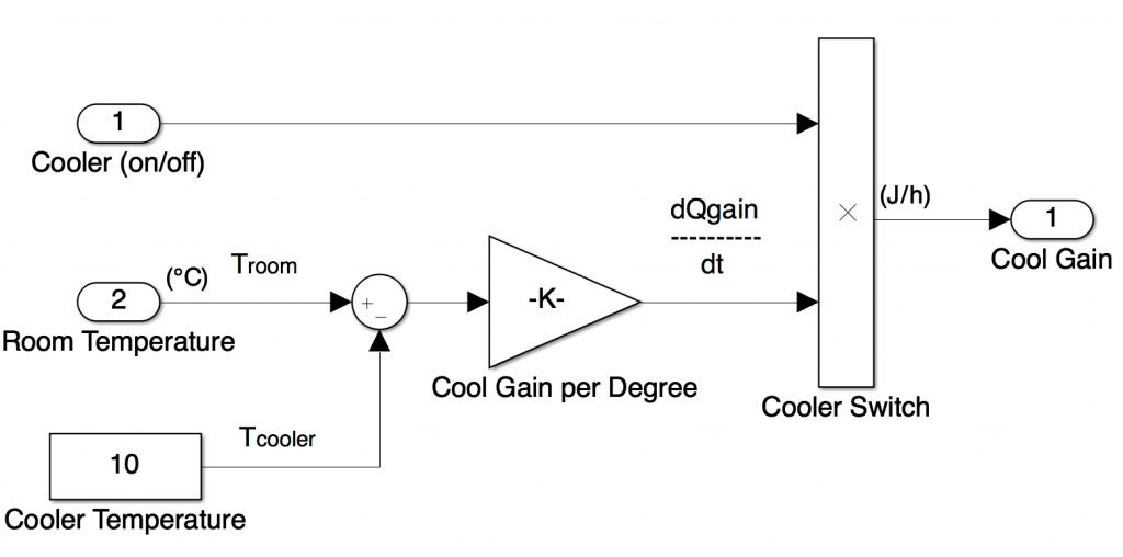
Figure 5 – Cooling Unit Sub-System
Cooling Unit Sub-System
Both heating and cooling unit sub-systems were created, however this section will only show how the cooling unit operates. The cooling unit sub-system takes the current temperature from the room and a control signal from the thermostat as its inputs and calculates the cool gain and outputs this when the room temperature is higher than the set point temperature after the signal is given from the thermostat. In order to model the cooling unit sub-system so that this is able to happen, Equation 3 can be altered to become Equation 8 as this will be for the cooling unit. This can be modelled with Simulink blocks as shown in Figure 5.

(8)
A constant block was added to the sub-system to model the constant air temperature from the cooler. There is also an inport block to enable the room temperature to be connected into the cooling unit. A sum block is then used so the cooler temperature can be subtracted from the room temperature. Once this has been calculated it must be multiplied by the cool gain per degree. A gain block is added to the sub-system and the output from the sum block is connected to it. To enable the thermostat to decide whether the cooler should be on or off, a switch must be used so the on/off signal from the thermostat to the cooler can trigger the cool gain per degree operation. A product block with two inports is used and the output from the cool gain per degree block is connected to one input whilst the cooler (on/off) function is connected to the other. The outport block created is entitled cool gain and will be connected the room sub-system. To ensure that the cooling unit sub-system would operate correctly, it was validated in a similar way to the validation of the thermostat sub-system by thinking about its expected behaviour.
Room Sub-System
The room component has two inputs, heat flow from the cooling unit sub-system and the outside air temperature. These inputs compute heat loss through the walls and the current room temperature. Equations 6 and 7 were used to design the room sub-system which is shown in Figure 6. Equation 9 is the rate of temperature change in the room where letters have been assigned to help understanding:

(9)
The term Y is a signal from the cooler and again, a sum block was used to calculate the difference between the cool gain and the loss with each being an input to the sum i.e. Y – Z. A gain block was added (X) to complete Equation 9 with the output of the gain block being the change in room temperature (W). In order to get the current room temperature, the signal required to be integrated which is why an integrator block has been added with an initial condition parameter set – TroomIC. The integrator block is then connected to the output which is room temperature.
To model the losses from the room, Equation 10 is given as the rate of thermal energy loss through the walls subtracted from the internal equipment load:
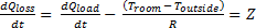
(10)
Another sum block was used to subtract the room temperature from the outside temperature. This occurred after another inport block was created for the outside temperature and connected to one of the inputs of the sum block whilst room temperature was the other. Another gain block was added in the opposite direction to model the thermal resistance and the internal equipment load. The output of this gain was then connected to the sum which also has the cool gain as an input, completing the loop. Note that in Figure 6 there is another sum block which incorporates both a heat gain and cool gain input prior to the one mentioned, this is for systems that require both heating and cooling as this is the gain from the heating unit and the gain from the cooling unit. To ensure that the room sub-system would operate correctly, it was validated by thinking about its expected behaviour through doing a trial simulation.
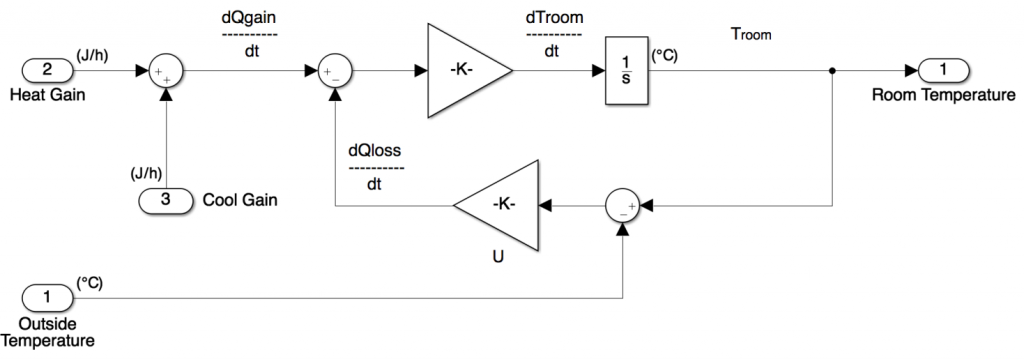
Figure 6 – Room Sub-system
Station Room System
The sub-systems are connected together in the orientation as shown in Figure 7 and the inputs and outputs of the sub-systems can be seen. The set point temperature value for both thermostats in this occasion is 20°C as can be seen by the constant blocks on the left hand side. The outside temperature input into the room sub-system is taken from data that is estimated to be the outside temperature of particular station rooms which will be modelled. The block entitled ‘Room Temperature’ on the right hand side enables output data to be recorded into a spreadsheet so that the data can be analysed. The antenna’s in the system signifies where data is obtained.
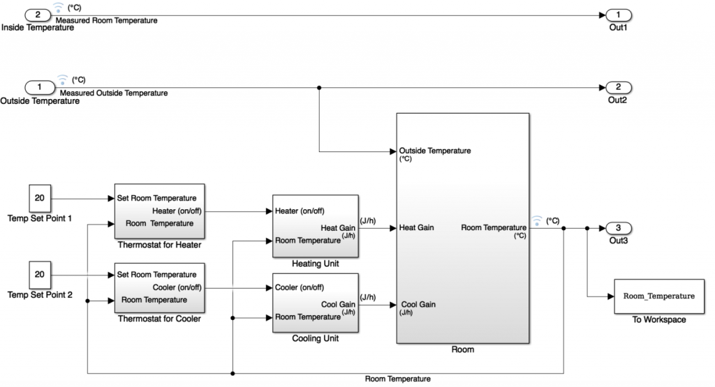
Figure 7 – Station Room System
5. Parametric Studies
In this section, two parameters are analysed by comparing a range of different values for them. The thermal conductivity of the room and the temperature of the cooler were assessed and while this occurred, all other parameters were kept constant. This was done to ensure that the correct values for each of these parameters would be chosen to enable the modelled system to be like a Crossrail station room.
5.1. Thermal Conductivity
Thermal conductivity is a material property which describes how good a material is at conducting heat. Thermal transmittance is known as the rate of transfer of heat energy through 1m2 of a structure, divided by the difference in temperature across the structure. Traditionally, well-insulated parts of a building have a low thermal transmittance. In this instance, it is expected that the Crossrail station rooms will have a very low thermal transmittance meaning that the outside temperature will have little effect on the inside room temperature and the main reason for the room to be heated up will be because of the internal equipment load.
Three different output responses of the system were conducted when the error deadband was kept constant but a different thermal conductivity value was used each time. As expected, when k decreases, the less the effect the outside temperature has upon the room temperature. When k is increased above the highest value selected, the room temperature and the outside temperature gradually become equal. This scenario would be if there are essentially no walls between the room and the outside. This was as expected because k is directly proportional to U. For a station room, the internal equipment load is going to have a much greater effect on the room temperature than the outside temperature. After conducting the analysis, a conductivity value of 1000 J/mhr°C was chosen for this reason.
5.2. Cooling Unit Temperature
The temperature that the cooling unit is set to was assessed as in the final results a constant value will need to be used when the error deadband is changed. Figure 8 shows the room temperature when the error deadband constantly stays as 3°C with the set point temperature being 20°C whilst the cooler temperature changes. When the temperature of the cooler is higher than the lower limit of the error deadband, then the cooler is going to be constantly switched on trying to cool the room to 18°C when it would be more energy efficient to let the temperature of the room fluctuate more between 17°C and 23°C. In contrast, having the cooler temperature exceedingly below the lower limit of the error deadband will mean that more energy will be used to reduce the temperature faster than necessary. Whereas, with the temperature of the cooler being just below the lower limit of the error deadband i.e. at 15°C, both the issues mentioned can be avoided. In the final results, a cooler temperature will always be used which is appropriately just below the value that is attempted to be cooled to.
Figure 8 – Cooler Temperature Parametric Study
6. Results and Discussion
In this section, the results of the simulated SER and SSO are shown and discussed. The values used for the simulations are written in Table 3 with the internal equipment load being kept constant. The main purpose of this analysis is to see the comparison of the response of the room temperature depending on the error deadband rather than the exact results due to the range of room sizes and internal equipment loads in rooms across the network. Each of the results take into account what the temperature limits are for that particular room in the new Crossrail stations and what the set point was in LU stations.
6.1. Signalling Equipment Room
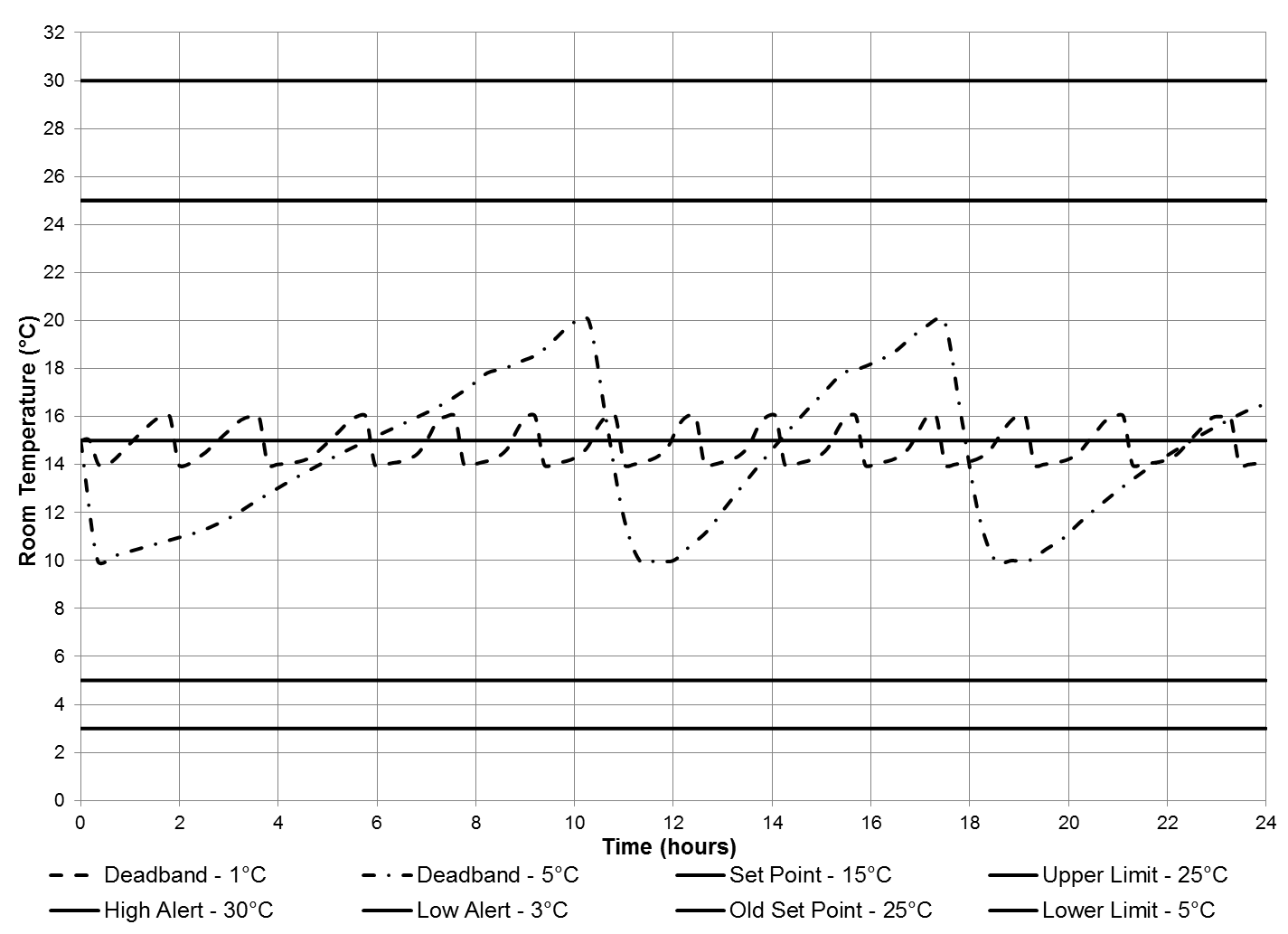
A simulation of the SER took place when the cooler temperature is kept constant for two different error deadbands and is shown in Figure 9. The set point temperature of an SER would change depending on the particular station but for now 15°C was chosen as it is directly in-between the upper and lower limits for the SER. Note that at the start of this simulation, the room is being cooled down to 10°C for the 5°C error deadbands.
The amount of cycles around the set point changes depending on what the error deadband is due to the cooler switching itself on at a lower temperature for the smaller error deadband after the room has heated up. For the error deadband of 1°C, there are 13 cycles and for 5°C, there are three cycles. The old set point can be seen to be at 25°C which had no error deadband at all. This would have meant that a lot of cooling would have been required to ensure that the temperature is kept constantly at 25°C, similarly to that of the set point temperature of 15°C with a 1°C error deadband. The total amount of cooling time is approximately 5.7 hours for the error deadband of 1°C but it reduces to three hours when the error deadband is increased to 5°C, which should reduce the amount of energy required to cool. The more frequent the cycles are means that cooling components are more at risk to fail from fatigue from expansion and contraction due to thermal stresses than when there is less temperature fluctuation. However, having an error deadband much larger could mean that the alert temperatures could be in danger of being reached which would be unsafe.

Figure 9 – A comparison between 2 different error deadbands used when simulating the room temperature of the SER
6.2. Station Supervisor’s Office
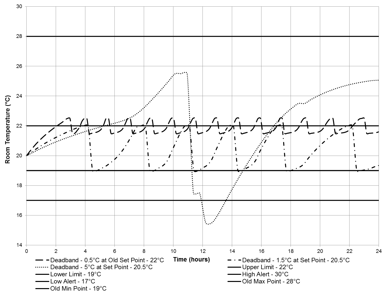
A simulation of the temperature response of the SSO when the cooler temperature is kept constant is shown in Figure 10. The set point for the SSO for Crossrail stations is 20.5°C with a much smaller error deadband compared to the SER – 1.5°C. Figure 10 shows the room temperature response when the error deadband changes from 1.5°C to 5°C for the set point of 20.5°C and also for an error deadband of 0.5°C at the set point of 22°C which was the old LU set point. For this, there are 13 cycles but for the error deadband of 1.5°C, there are six cycles. This reduction in the number of cycles is beneficial similarly to the SER. However, increasing the error deadband to 5°C around the set point of 20.5°C, means that there is only one temperature cycle but unfortunately this large fluctuation in temperature would cause there to be too much discomfort for the people working in the room so is not an option despite the likely energy saving.
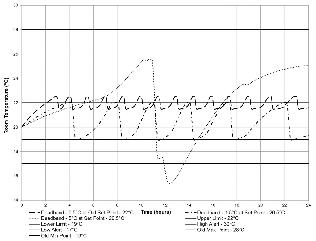
Figure 10 – A comparison between different error deadbands used with the new set point temperature of Crossrail SSOs
7. Energy Savings Calculation
This section was conducted to compare the differences in energy used during cooling between having a cooling unit set with a larger error deadband compared to a smaller one for the SER. It was decided that the losses in temperature (Qloss) when comparing different error deadbands for the cooling units were deemed to be negligible and the time and temperature readings taken for each cooling cycle from the same simulation were the same. Table 4 shows the percentage energy saving during cooling between having an error deadband of 1°C and 10°C for the proposed cooling units in the SER. Equation 11 calculates the energy used during cooling in kWh for the SER with a 5°C error deadband which can be seen to require 12.3% less energy during cooling if the error deadband is 5°C compared to 1°C. Note that this calculation does not take into account the amount of energy required to switch on the cooler each time, which is likely to be directly proportional to the number of cycles. For the SER, the cooler will require to be switched on 10 more times per day compared to when a larger error deadband is used.

(11)
Table 5 shows the percentage of energy saved from the amount of energy which is given to HVAC to cool one station each day if an error deadband of 5°C is used instead of 1°C for the cooler in the SER. An estimated figure for the total electricity consumption for the eight underground stations in the Crossrail Central Section was taken from a Building Research Establishment Environmental Assessment Method (BREEAM)[9]. The estimated apportionment given to HVAC is 30%. Table 5 shows that the 12.3% of energy saved from increasing the size of the error deadband equates to a difference of 0.12% in the percentage of energy saved from the HVAC apportionment. This is only for the SER so there could be even more potential savings if this was done to all rooms which have large internal equipment loads.
Table 4 – Energy Saving Calculation for the SER
Room SER Error Deadband (°C) 1 5 Difference between start of cooling and the cooler Temp (°C) 6 10 Total Cooling Time (hr) 5.7 3.0 Cool Gain per Hour (MJ/hr) 21.72 36.19 Energy Used during Cooling (kWh) 34.38 30.16 Percentage Energy Saving during cooling between the two error deadbands 12.3% Table 5 – Energy saved from the HVAC apportionment because of the SER
Annual Electricity Consumption for the Central Underground Crossrail Stations (GWh) 35.6 Number of Central Underground Stations 8 Annual Electricity Consumption per Station (GWh) 4.4 HVAC Contribution to Annual Energy Usage 30% HVAC Annual Energy Apportionment per Station (GWh) 1.33 HVAC Daily Energy Apportionment per Station (MWh) 3.654 Difference in daily energy use in the SER when different error deadband is used (kWh) 4.22 Percentage of energy saved from the HVAC apportionment to cool the SER daily with a 5°C error deadband compared to a 1°C error deadband 0.12% 8. Conclusion
This paper has shown that the implementation of larger error deadbands for temperature controllers in the new Crossrail stations will be beneficial in reducing the number of on/off cycles of the cooling equipment. Cooling components will be less at risk to fail from fatigue due to thermal stresses. This followed analyses of 2 rooms – the SER and the SSO. As expected, for the SER, the cooling time was approximately halved when the larger error deadband was used with 12.3% less energy required to cool the room per day. More energy would likely be saved also as the cooler would be turned on 10 times less per day compared to having a smaller error deadband. Table 6 summarises the performance benefits of increasing the error deadband or elevating the set point temperature.
Although this report has highlighted the benefits in having a wider error deadband than previously designed, the ability of being able to adjust the set point temperature and the on-field error deadband could be very useful. Currently, BMS and CCU controllers do allow for adjustments, but there are limitations on the implementation of this in other rooms because of some of the proprietary controllers not allowing on-field adjustment of the error deadband, (see Table 1). Enabling more controllers to have the ability to adjust the on-field deadband would produce energy benefits. Three different sources were found which detail products which are able to both adjust their temperature set point and on-field error deadband and are recommended to be researched further for application into station room designs in the future[13] [14] [15].
It is to be noted that a rather crude model was used and the results can only be used for use of qualitative description of system performance of the temperature controllers. However, the results indicate that by suitable adjustment of error deadband, the problem of undue on-off cycling of the cooling plant can be avoided. This is at the expense of and increased room temperature fluctuations. On the other hand, while adjustment of the room set point will lead to a reduced cooling load, it may also lead to frequent cycling which may reduce the system working life.
Table 6 – Comparison of having an elevated Set Point to an increased error Deadband
Larger and fewer fluctuations in room temperature Reduction in the Cooling Energy needed Improved working life for cooling plant Elevated room set point temperature No Yes, there is a small reduction No Increase in the size of the error deadband Yes Yes, as the higher heat gain at lowered room temperature is offset by lower room temperature as the room temperature swings with an increase in error deadband Yes, because of the reduction in the numerous on/off cycles which occur with a smaller error deadband References
[1] “Control Fundamentals,” in CIBSE Guide H: Building control systems, CISBE, 2009. [2] S. Norman, “Analysis and Design Objectives,” in Control Systems Engineering 6th Edition, John Wiley & Sons (Asia) Pte Ltd, 2011, pp. 10-11. [3] Danaher Industrial Controls Group – Process Automation, Measurement, & Sensing, “Temperature Controller Basics Handbook,” 2010. [4] D. Shetty and R. Kolk, “Chapter 7: Signals, Systems and Controls,” in Mechatronics System Design 2nd Edition, Global Engineering: Christopher M. Shortt, 2011, p. 330. [5] G. Mansen, Sheffield University: MEC319: Controllers, Sensors and Actuators, 2014. [6] CarbonTrust, “Understanding and using Controls,” in Heating, Ventilation and Air Conditioning, 2011, pp. 11-13. [7] Strategic Rail Consultants, “Equipment Room Development and Design,” London, 2012. [8] S. Duffy, “Supporting Information,” in S1068 – Mechanical Building Services, Utility Provision and Energy Management in LU, London, 2015, pp. 33-38. [9] W. Fung, Electricity Consumption for the Reference Station, London, 2017, pp. 16-18. [10] MathWorks, “MathWorks Support,” 2017. [Online]. Available: https://uk.mathworks.com/help/matlab/ref/help.html. [11] MathWorks, “Model a Dynamic System,” Mathworks, 2017. [Online]. Available: https://uk.mathworks.com/help/simulink/gs/define-system.html?requestedDomain=www.mathworks.com&requestedDomain=uk.mathworks.com. [12] M. David, “Commissioning Set Points – Room Temperatures,” London, 2017. [13] Airedale, “Downflow and Upflow – Precision Air Conditioning,” 2016. [14] Honeywell, “ComfortPoint Open BMS: Specification & Technical Data,” Golden Valley, 2012. [15] Mitsubishi Electric, “MA Remote Control Instruction Book,” Tokyo, 2012. -
Authors

Harry Morgan MEng Eng Tech MIMechE MPWI - Crossrail Ltd
Harry Morgan was a Graduate Mechanical Engineer at Crossrail providing mechanical engineering support to the Chief Engineers Group until October 2017. He is currently employed by Transport for London and had a secondment with Crossrail for 4 months and it is during this time that he was able to write this technical paper. Harry completed his Mechanical Engineering degree with the University of Sheffield in 2016 and had experience working for Transport Systems Catapult for the two summers before joining TfL in September 2016.

Wing Fung PhD MSc BSc(Eng) CEng MCIBSE - Arcadis
Technical Director (MEP), Arcadis
Wing is is a Chartered Engineer with over 30 years’ experience as a technical specialist engaged in mass transit system planning, design, project management, technical assurance, commissioning, energy management, operation and maintenance, and asset renewal. Wing has been with the Crossrail project in the CRL Chief Engineer Group since 2013, overseeing mechanical design, systems integration and T&C.
Specialties: Building Services, Mechanical Engineering, Computational Fluid Dynamics, RAM studies, Systems Integration, Requirement Management, Testing and Commissioning.