Notation

D	Axial separation
d	Tunnel diameter
EB	Eastbound
GRP	Ground Response Program
HF	Harwich Formation
i	Distance from tunnel centreline to the point of inflexion on a settlement trough
JLE	London Underground Jubilee Line Extension
K	Trough width factor
LC	London Clay
LG	Lambeth Group
LHS	Left hand side
MG	Made Ground
m	Meters
mm	Millimetres
No	Number
kPa	Kilopascal
RHS	Right hand side
RTD	River Terrace Deposits
S	Surface settlement
SCL	Sprayed concrete lined
Smax	Maximum settlement
S,Solver	Surface settlements produced by the mathematical function using Solver (curve fitting)
TBM	Tunnel boring machine
TS	Thanet Sands
VF	Excavated volume of tunnel face per m
VL	Volume loss
Vs	Volume of settled material per m
VS,trap	Volume of settled material per m confined underneath the S,Solver points and found using the trapezium rule
WB	Westbound
x	Distance along the tunnel parallel to its axis
y	Transverse distance from the tunnel centreline
Z	Depth of tunnel axis below ground level
Σ	Sum

 

Introduction

The Stepney Green Crossrail site contains a box shaft connected to two underground sprayed concrete lined tunnels (eastbound and westbound). The eastbound and westbound SCL tunnels comprise large SCL caverns (up to 13.7 m high and 16.9 m wide). The eastbound and westbound tunnels include lengths of tunnel with a reduced diameter, located where TBMs were received at Stepney Green, and re-launched from the site to create running tunnels.

The Stepney Green eastbound cavern will provide the junction where Crossrail trains can travel towards Shenfield or Abbey Wood, and the westbound cavern will receive passengers travelling from Shenfield and Abbey Wood.

Mott MacDonald was the SCL permanent works designer and contractors Dragados Sisk Joint Venture (DSJV) undertook the construction. OTB Engineering provided the DSJV with the temporary works design and WJ Groundwater implemented the dewatering systems. Instrumentation and monitoring of ground settlement was carried out by Geocisa UK.

During the design process of the underground structures at Stepney Green, empirical predictions of surface settlement were carried out. This is an important part of any tunnelling project, as it gives an indication of the expected impact on infrastructure and urban society.

During the construction process, surface settlement was measured using levelling points. The data from the levelling points gives an indication of what is actually happening to the surface during each construction stage of the underground structures.

Measured surface settlement data can then be used to identify the shape of the settlement profile and interpret the volume loss of ground material due to tunnel construction, allowing for prediction verification.

The aims of this paper are:

• To assess the shapes of the settlement profiles to interpret the volume loss of ground material due to SCL tunnel construction at the Crossrail Stepney Green site.
• To compare the measured values with predicted surface settlement (and volume loss) values, for the land above underground Crossrail SCL tunnelling at Stepney Green.
• To consider the impact of dewatering on ground settlement at the Crossrail Stepney Green site.

This investigation uses measured data representative of when excavation and primary SCL works had been completed for the eastbound and westbound SCL tunnels at Stepney Green. At Stepney Green there are three transverse arrays of levelling points situated on the ground surface above the SCL tunnels. This paper considers three different SCL cross-sections for the eastbound and westbound tunnels.

Stepney Green Site

Site geology

Figure 1 and Figure 2 are geological long sections for the eastbound and westbound tunnels. From Figure 1 it can be seen that the eastbound tunnel is located completely within the London Clay (predominantly A2 unit), with the tunnel invert resting on top of the Lambeth Group. The London Clay at Stepney Green is firm to very stiff, with the A2 unit having an increase of silt partings ^[1]. However, Figure 2 shows that the westbound tunnel is situated at a depth approximately 5 metres lower than the eastbound tunnel, resulting in the top half of the westbound tunnel being in the London Clay (A2 unit), with the bottom half of the tunnel located within the Lambeth Group.

Figure 1 – Geological long section for eastbound tunnel

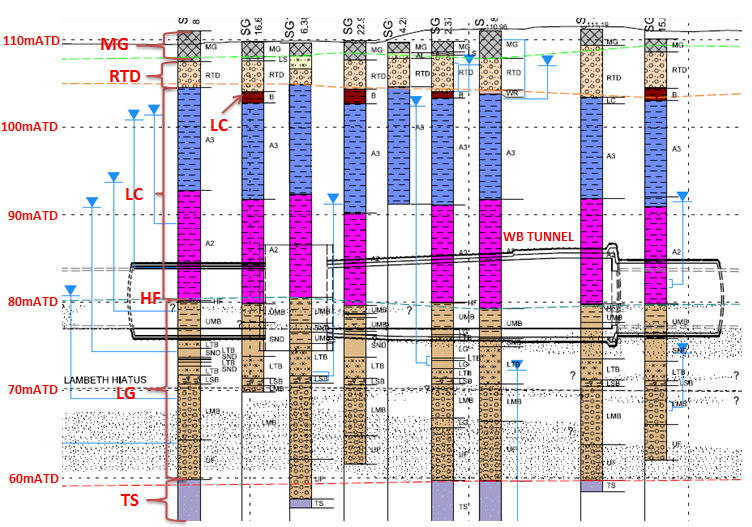
Figure 2 – Geological long section for westbound tunnel

Dewatering at Stepney Green site

Geological research of the Stepney Green site during the desk study stage revealed the presence of sand channels in the Harwich Formation and the upper regions of the Lambeth Group (i.e. the Upper Mottled Beds, Laminated Beds and Lower Shelley Beds). The water-bearing properties of sand and the Lambeth Group gave pore water pressures of up to 150 kPa in the Harwich Formation and 220 kPa in the Lambeth Group sand channels ^[2]. This meant dewatering would be required prior to and during excavation works at Stepney Green in order to lower the groundwater levels to depths below tunnel invert levels to ensure safe tunnel excavation.

Figure 3 shows the layout for the surface ejector wells used for dewatering at Stepney Green. In total, 45no surface ejector wells were drilled, of which 27no were vertical, and 18no were inclined (in order to dewater areas on site where surface ejector wells could not be placed).

Although surface ejector wells were able to lower the groundwater level below eastbound tunnel inverts, it was not sufficient for the westbound tunnel which is situated 5m deeper. Therefore in-tunnel pumping was required to target the areas not adequately drained by the surface ejector wells, to bring the water table below the tunnel inverts for the westbound tunnel.

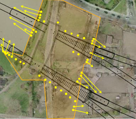
Figure 3 – Plan view of Stepney Green site showing the location of surface ejector wells ^[2]

Crossrail works at Stepney Green

Overview of works

The eastbound and westbound SCL tunnels at Stepney Green have been divided into sections A-G.

Figure 4 is a plan view of the SCL works at Stepney Green. The lengths of the SCL tunnels and the locations of sections A-G are labelled in Figure 4. Numbers 1-4 refer to the order of excavation works (see Table 1 and Table 2).

Figure 5 is another plan view of Stepney Green. In Figure 5, the dashed arrows represent TBM drive Z and the solid arrows represent TBM drive Y. The TBM paths are also labelled 1 to 6, representing the arrival/re-launch sequence of the Stepney Green TBMs. Table 3 summarises the arrival/ re-launch sequence of Stepney Green TBMs.

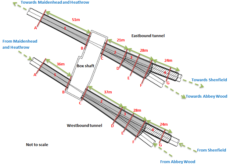
Figure 4 – Plan view of SCL works at Stepney Green

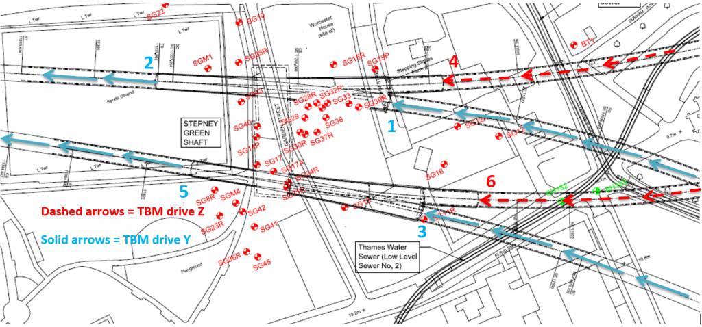
Figure 5 – Plan view of Stepney Green, with TBMs shown in solid and dashed arrows and labelled 1 to 6 indicating arrival/re-launch sequence

Excavation sequences overview for SCL tunnels at Stepney Green

Table 1 and Table 2 summarise the order of excavation works for the eastbound and westbound SCL tunnels at Stepney Green, with part 1 being excavated first for each tunnel. Excavation works for the eastbound tunnel started before the westbound tunnel and note that excavation stoppage dates have not been included in Table 1 and Table 2.

Table 1 – Summary of excavation sequence for the eastbound tunnel at Stepney Green

Part	Description	Excavation sequence	Excavation dates
1	51 m of SCL tunnel spanning section A to section B	Top heading, bench then invert excavation (see Figure 6 for an example).	Started on 28.11.12, finished on 11.1.13.
2	21 m of SCL tunnel spanning section C to section D	Top heading, bench and invert excavation of left side of tunnel before breakout of temporary sidewall to excavate top heading, bench and invert of right side of tunnel (see Figure 7 for an example).	LHS: started on 12.1.13, finished on 24.2.13. RHS: started on 3.2.13, finished on 17.3.13.
3	28 m of SCL tunnel spanning section D to section F (with section E located between D and F)	Top heading, bench and invert excavation of left side of tunnel before top heading, bench and invert excavation of right side of tunnel. Following this top heading, bench and invert excavation occurs for the centre drift, ending with breakout of temporary sidewall (see Figure 8 for an example).	LHS: started on 22.2.13, finished on 7.4.13. RHS: started on 14.3.13, finished on 3.4.13. Central drift: started on 7.4.13, finished on 13.5.13.
4	24 m of SCL tunnel (with section G consistent in geometry for the whole span)	Top heading, bench then invert excavation.	Started on 16.5.13, finished on 1.6.13.

 

Table 2 – Summary of excavation sequence for westbound tunnel at Stepney Green

Part	Description	Excavation sequence	Excavation dates
1	36 m of SCL tunnel spanning section A to section B	Top heading, bench then invert excavation.	Started on 2.2.13, finished on 6.3.13.
2	37 m of SCL tunnel spanning section C to section D	Top heading, bench and invert excavation of left side of tunnel before breakout of temporary sidewall to excavate top heading, bench and invert of right side of tunnel.	LHS: started on 7.3.13, finished on 6.5.13. RHS: started on 5.4.13, finished on 11.6.13.
3	28 m of SCL tunnel spanning section D to section F (with section E located between D and F)	Top heading, bench and invert excavation of left side of tunnel before top heading, bench and invert excavation of right side of tunnel. Following this top heading, bench and invert excavation occurs for the centre drift, ending with breakout of temporary sidewall.	LHS: started on 2.5.13, finished on 26.5.13. RHS: started on 8.6.13, finished on 10.7.13. Central drift: started on 10.7.13, finished on 11.8.13.
4	24 m of SCL tunnel (with section G consistent in geometry for the whole span)	Top heading, bench then invert excavation.	Started on 15.8.13, finished on 29.8.13.

Note that section D is at the intersection between two lengths of tunnels with different excavation sequences. Therefore section ‘D1’ (which is just west of section D) has the same excavation sequence as section C, however section ‘D2’ (which is just east of section D and is connected to the length of tunnel leading to section E) has the same excavation sequence as sections E and F.

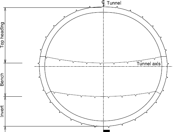
Figure 6 -Excavation sequence for tunnel spanning section A to B and section G (parts 1 and 4)

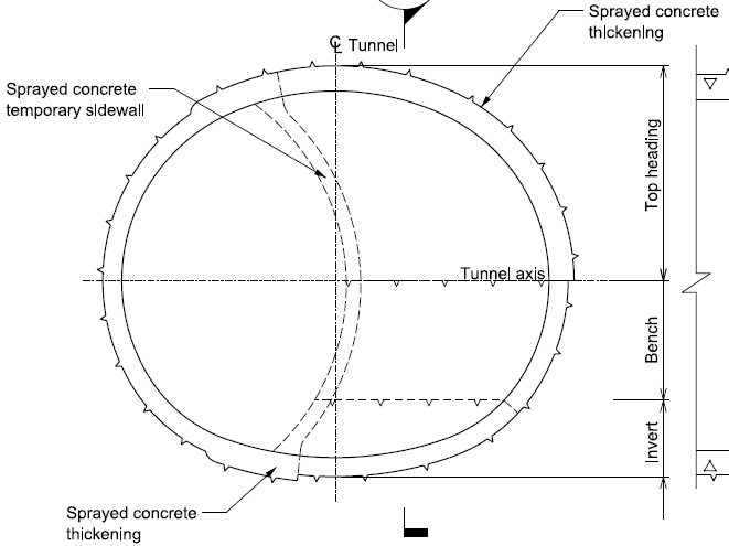
Figure 7 – Excavation sequence for tunnel spanning section C to D1 (part 2)

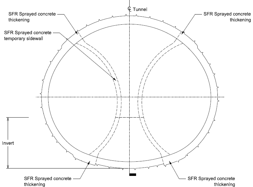
Figure 8-Excavation sequence for tunnel spanning sections D2 to F including section E (part 3)

Stepney Green TBM arrival and re-launch dates

Table 3 summarises the order of arrival/re-launch for TBM drives Y and Z at Stepney Green, shown on Figure 5.

Table 3 – Summary of TBM arrival/re-launch dates at Stepney Green

No.	Description	Date
1	TBM drive Y arriving at EB tunnel	Arrived on 6.11.13
2	TBM drive Y re-launched from EB tunnel	Re-launched on 21.11.13
3	TBM drive Y arriving at WB tunnel	Arrived on 30.1.14
4	TBM drive Z arriving at EB tunnel	Arrived on 3.2.14
5	TBM drive Y re-launched from WB tunnel	Re-launched on 22.2.14
6	TBM drive Z arriving at WB tunnel	Summer 2014

 

Eastbound and westbound SCL cross-sections

Table 4 summarises the dimensions of the eastbound and westbound SCL sections.

Table 4 – Summary of sizes for SCL sections at Stepney Green

Section	Tunnel	Max height (m)	Max width (m)	VF (m3/m)
A	EB	8.750	8.130	54.633
A	WB	8.645	7.980	54.633
B	EB	8.905	9.525	65.958
B	WB	8.645	7.980	54.633
C	EB	10.055	11.348	83.272
C	WB	8.599	9.869	70.790
D	EB	11.429	13.241	120.013
D	WB	11.224	12.953	120.013
E	EB	12.598	15.004	139.870
E	WB	12.598	15.004	139.870
F	EB	13.679	16.919	180.387
F	WB	13.679	16.919	180.387
G	EB	8.645	7.980	54.633
G	WB	8.645	7.980	54.633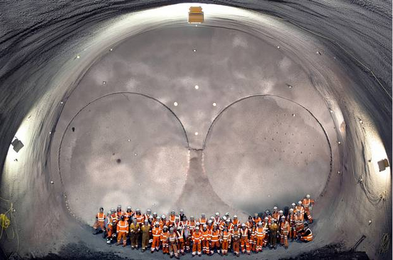

 

Figure 9 – Photograph of section F for the EB tunnel^[3], showing the large size of the SCL section

Instrumentation and monitoring

Geocisa UK used levelling points to monitor the surface settlement caused by underground construction. The levelling points are located in arrays longitudinal and transverse to the eastbound and westbound tunnels.

Analytical Procedures

Levelling points and cross-sections selected for investigation

Overview of selected arrays

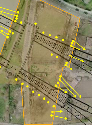
Three arrays of levelling points (Arrays 1, 2 and 3) are situated transversely above the SCL tunnels at Stepney Green. Figure 10 is a plan view of the site showing Stepney Green levelling points, with the levelling points used in this investigation circled.

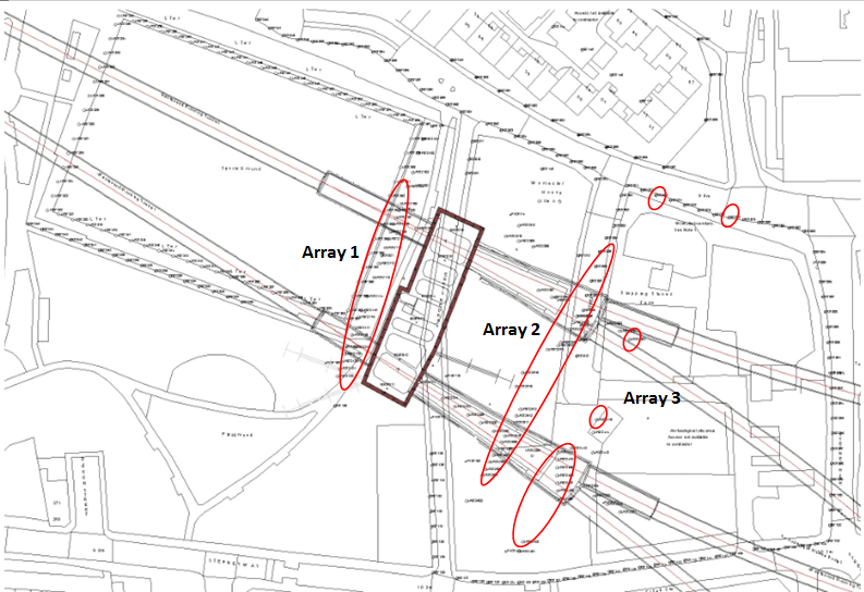
Figure 10 – Plan view of Stepney Green with levelling points used in the investigation for SCL tunnels circled

Figure 11 shows the Stepney Green tunnels, and the straight lines connect the levelling points used. The SCL tunnels are outlined with solid lines and TBM tunnels are outlined with dashes. Section G on Array 3 has levelling points located far from the actual SCL section (as can be seen in Figure 10 and Figure 11), but to have a long array of levelling points spanning both tunnels, this section was included.

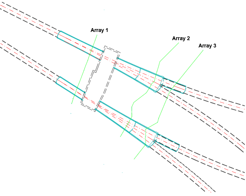
Figure 11 – Plan view of Stepney Green with levelling points used in this investigation connected with solid lines

Overview of SCL sections

Table 5 summarises the SCL sections considered. Appendix A.1 details the specific levelling points and dates of measurement, as well as the interpolation calculations to find the volume of the excavated face for each section, V_F (m³/m). Although the SCL sections are not completely circular, the ‘equivalent diameter’ for each section is also presented in Table 5 (back calculated from the values of V_F, assuming the sections are circular).

Table 5 – Summary of SCL sections

Section	VF (m3/m)	D (m)
Array 1, WB tunnel	54.633	8.340
Array 1, EB tunnel	62.561	8.925
Array 2, WB tunnel	115.091	12.105
Array 2, EB tunnel	162.275	14.374
Array 3, WB tunnel	159.256	14.240
Array 3, EB tunnel	54.633	8.340

Accounting for dewatering induced surface settlement

Since dewatering continued during the excavation works for the SCL tunnels, it is difficult to separate the surface settlement caused by dewatering from that due to tunnel excavation. Instead, surface settlement caused by surface well dewatering (prior to excavation of tunnels) was plotted, and deducted from the surface settlement measured from levelling points on the dates presented in Appendix A.1. Appendix A.2 shows the levelling points and dates used to obtain dewatering induced settlement (before excavation works for the tunnels commenced).

Methodology for assessing surface settlement

The method adopted for assessing surface settlement at Stepney Green is presented in a series of steps.

Step 1 – determining distances between levelling points and axial separation of parallel tunnels

Appendix B.1 summarises the location of tunnel centrelines with respect to neighbouring levelling points. Appendix B.1 also shows the axial separations and total length of each of the arrays (i.e. total cumulative straight-line distance between points in an array).

Step 2 – obtaining surface settlement readings for levelling points and accounting for dewatering induced surface settlement

Once the surface settlement readings (for the measurement dates presented in Appendix A.1) were recorded, dewatering induced surface settlement was then deducted from each point using data from the dates in Appendix A.2. This allowed the plotting of the excavation-induced surface settlement along each array.

Step 3 – curve fitting to measured data using Solver in Excel

Solver (Excel Add-In) can be used to maximise, minimise or find an exact value of a specific cell, by changing the values of variables that are located in other cells. Appendix B.2 summarises the procedure of using Solver to produce a best fit curve for the measured data (i.e. the levelling point data).

Parallel tunnels surface settlement function

In 1991, New and O’Reilly described the surface settlement caused by twin tunnels as:

 

(1)

In Equation 1, S_y,x is the vertical surface settlement caused by the twin tunnels, V_s is the settlement volume per unit advance of the tunnels, and D is the axial separation of the tunnels ^[4]. Equation 1 assumes that both tunnels have the same tunnel diameter, volume loss and trough width and does not account for interaction between the two tunnels ^[5]. Figure 12 is a diagram of the transverse settlement trough caused by twin tunnels.

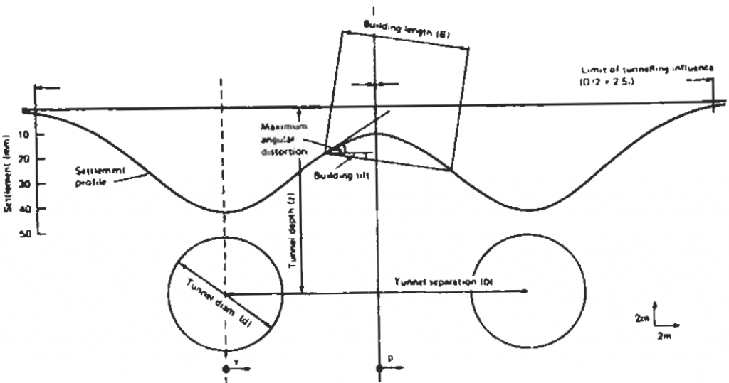
Figure 12 – Transverse settlement profile of twin tunnels ^[4]

If parallel tunnels do not have the same diameter, ground loss or trough width, the following equation can be used to model the transverse surface settlement (presented by Wang et al in 2003):

 

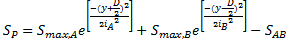(2)

In Equation 2: S_P is the vertical surface settlement caused by the parallel tunnels; S_max,A is the maximum settlement caused by tunnel ‘A’; y is the transverse distance from the centreline of the parallel tunnels; D is the axial separation, S_max,B is the maximum settlement caused by tunnel ‘B’;  i_A and i_B are the distances from the tunnel centrelines to the points of inflexion on the curve for tunnels ‘A’ and ‘B’ respectively, and S_AB is not equal to zero if there is interaction between the parallel tunnels ^[6]. Equation 2 was the mathematical function used in the Solver curve fitting procedure and S_max,A, i_A, S_max,B, i_B and S_AB were defined as the changing variables.

Methodology for assessing volume loss

Appendices B.3 and B.4 contain descriptions of the two methods used to calculate the volume loss of each tunnel under investigation. Method 1 is based on the principles described by O’Reilly and New in 1982 and Method 2 involves calculating the volume of settlement confined by the best fit curve using the trapezium rule.

Predicted data for surface settlement and volume loss

Ground Response Program is a program developed by Mott MacDonald that can predict vertical and horizontal movements of the ground caused by underground works such as tunnels, shafts and open cuts. Appendix B.5 outlines the inputs required for GRP and the vertical settlement equation used for predictions.

For the empirical predictions for SCL tunnels at Stepney Green, volume losses were set at 1.5%, K was set to 0.5, and a point sink analysis was assumed hence ribbon widths were set to 0. A discussion on how the values of volume loss and K obtained from the measured data compare with these GRP inputs is provided later in this paper.

In order to compare measured settlement along the three arrays with predicted, line analyses were performed along the three SCL arrays in GRP, with GRP calculating vertical surface settlement at 0.05 m intervals along the line.

Figure 13 shows the Stepney Green tunnels with the GRP lines used for analyses shown by the dashed lines, and the levelling points used in the analyses connected with solid lines. The objective was to have GRP line analyses that went through a majority of levelling points along an array, for better comparisons of settlement to be made.

 

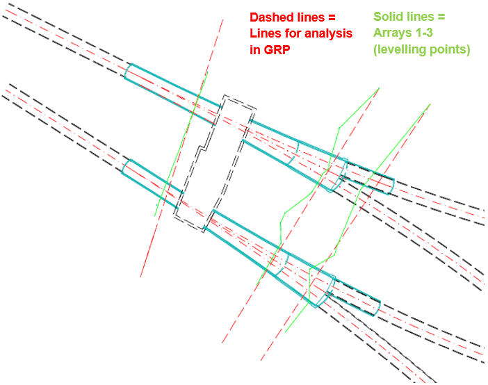
Figure 13 – Plan view of Stepney Green with GRP lines for analyses shown by the dashed lines and levelling points used in this investigation connected with solid lines

 

SCL Results

Note that for all settlement plots in in this chapter, the westbound tunnel is on the left and the eastbound tunnel is on the right. Also note that the points represent data from levelling points and the best fit curves can be seen by the solid curves. The dashed curves in this chapter represent empirical settlement predicted by GRP.

For each array, a table is provided summarising values of volume loss, K and S_AB. Note that the chosen volume loss values for each array from the two methods are presented in bold. Appendices C.1, C.2 and C.3 contains the full results tables for Arrays 1, 2 and 3 respectively.

Array 1

Measured and predicted settlement curves

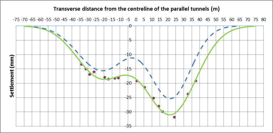
Figure 14 – Array 1 levelling point data (dewatering not accounted for) with best fit curve and predicted curve

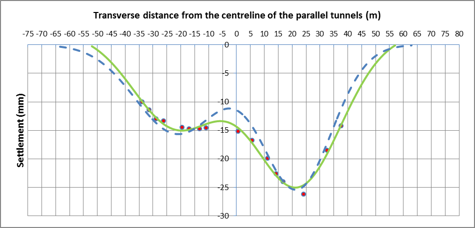
Figure 15 – Array 1 levelling point data (dewatering accounted for) with best fit curve and predicted curve

Array 1 results

Table 6 – Summary of Array 1 results

	WB tunnel	EB tunnel	Total
Method 1 (based on Smax1), VS1 (m3/m)	0.63	1.06	1.69
Method 1 (based on Smax1), VL1 (%)	1.2	1.7	–
Method 1 (based on Smax2), VS2 (m3/m)	0.58	0.99	1.57
Method 1 (based on Smax2), VL2 (%)	1.1	1.6	–
Method 2, VS (m3/m)	0.51	0.92	1.43
Method 2, VL (%)	0.9	1.5	–
Trough width factor, K	0.51	0.63	–
Interaction term, SAB (mm)	2.1		–

For the Method 1 calculations, S_max1 is greater for both tunnels in comparison to S_max2 (see Appendix B.3 for general descriptions of S_max1 and S_max2), hence V_L1 values are greater than V_L2 values. The Method 1 V_L1 values are also greater than the Method 2 volume losses and for conservativeness, the Method 1 V_L1 values are the chosen volume loss values for the tunnels (presented in bold in Table 6). The average volume loss of the chosen values is 1.5%, which is equal to the empirical prediction.

In Figure 15, the best fit curve has a steeper gradient at both ends of the settlement trough in comparison to the predicted curve and the two curves in Figure 14 (which appear to flatten out at the ends as expected of Gaussian profiles). Method 2 determines the volume of settled material per m directly from the material confined by the points along the best fit curve (using the trapezium rule). Therefore, the lack of flattening at the ends of the best fit curve in Figure 15 may have resulted in the total V_S for Method 2 to be smaller than the Method 1 V_S values.

Array 2

Measured and predicted settlement curves

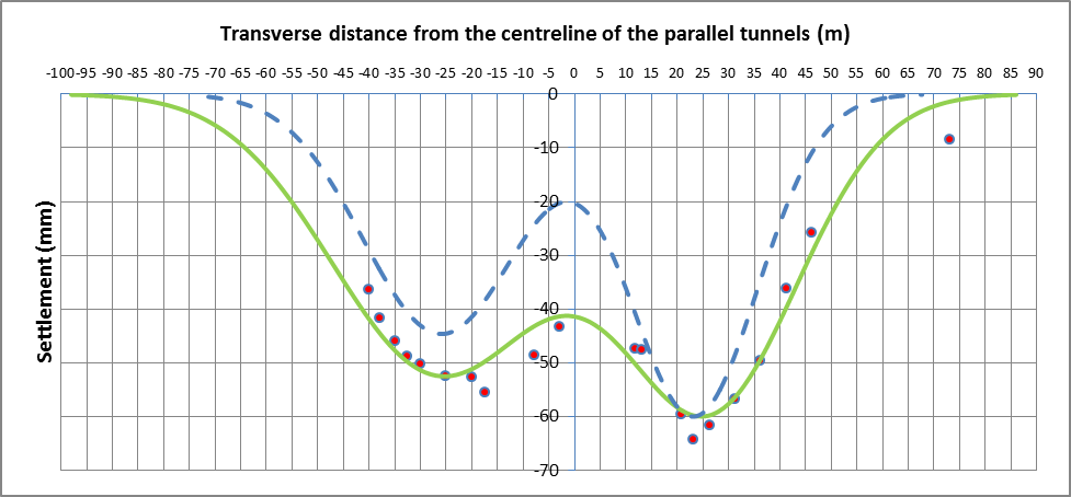
Figure 16 – Array 2 levelling point data (dewatering not accounted for) with best fit curve and predicted curve

 

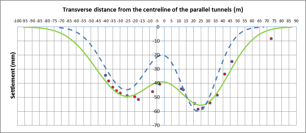
Figure 17 – Array 2 levelling point data (dewatering accounted for) with best fit curve and predicted curve

Array 2 results

Table 7 – Summary of Array 2 results

	WB tunnel	EB tunnel	Total
Method 1 (based on Smax1), VS1 (m3/m)	2.42	2.33	4.75
Method 1 (based on Smax1), VL (%)	2.1	1.4	–
Method 1 (based on Smax2), VS2 (m3/m)	2.46	2.41	4.87
Method 1 (based on Smax2), VL2 (%)	2.1	1.5	–
Method 2, VS (m3/m)	2.29	2.57	4.86
Method 2, VL (%)	2.0	1.6	–
Trough width factor, K	0.65	0.72	–
Interaction term, SAB (mm)	0.0		–

For Method 1, S_max2 is greater for both tunnels in comparison to S_max1, resulting in V_L2 values being greater than V_L1 values (V_L2 values being the more conservative choice of the two Method 1 sets). The average Method 1 V_L2 value of 1.8% is also equal to the average Method 2 volume loss. Since the WB tunnel has a greater volume loss than the EB tunnel, Method 1 V_L2 values are the chosen volume loss values for the individual tunnels (presented in bold in Table 7) as this is more conservative for the WB tunnel.

Array 3

Measured and predicted settlement curves

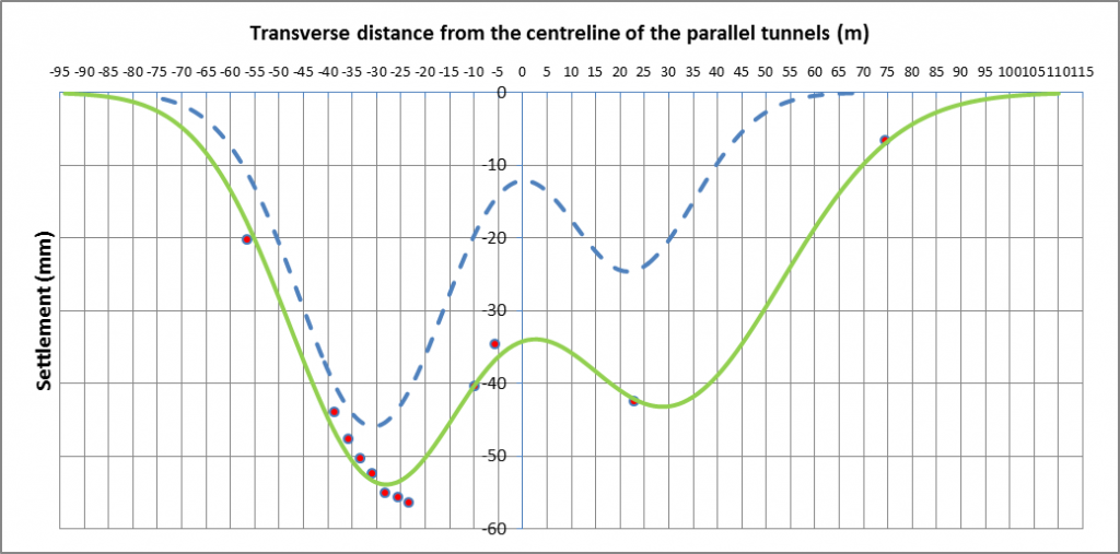
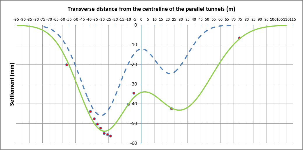
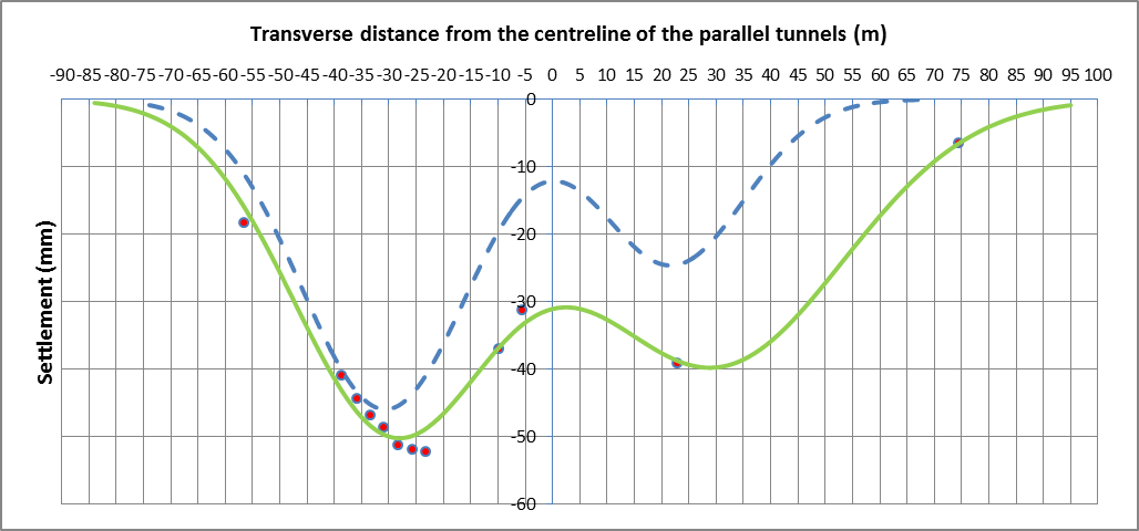
Figure 18 – Array 3 levelling point data (dewatering not accounted for) with best fit curve and predicted curve

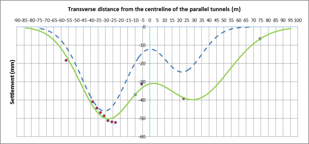
Figure 19 – Array 3 levelling point data (dewatering accounted for) with best fit curve and predicted curve

Array 3 results

Table 8 – Summary of Array 3

	WB tunnel	EB tunnel	Total
Method 1 (based on Smax1), VS1 (m3/m)	2.10	2.35	4.45
Method 1 (based on Smax1), VL (%)	1.3	4.3	–
Method 1 (based on Smax2), VS2 (m3/m)	2.19	2.36	4.55
Method 1 (based on Smax2), VL2 (%)	1.4	4.3	–
Method 2, VS (m3/m)	2.16	2.38	4.54
Method 2, VL (%)	1.4	4.3	–
Trough width factor, K	0.58	0.95	–
Interaction term, SAB (mm)	0.0		–

For the Method 1 calculations, S_max2 is greater for both tunnels in comparison to S_max1, resulting in V_L2 being greater than V_L1 for the WB tunnel but not for the EB tunnel. The volume losses of 1.4% and 4.3% for the WB tunnel and EB tunnel are consistent for both Method 1 V_L2 values and Method 2, hence these are the chosen values for array 2. The 4.3% volume loss for the EB tunnel can be ignored. This is because the lack of levelling points above the tunnel is likely to have caused the best fit curve to over-calculate settlement in areas where there were no levelling points.

The best fit curve above the WB tunnel has greater settlements and a larger i value in comparison to the GRP curve, yet the observed volume loss for this tunnel is less than the 1.5% empirical prediction. From Figure 13, it can be seen that the levelling points cut diagonally across the GRP line section. This brings the possibility that the measured data and GRP are presenting volume loss values for sections of the tunnel that are not identical in size.

Summary of SCL results

Table 9 – Summary of SCL results

Section	VF (m3/m)	D (m)	K	VL (%)
Array 1, WB tunnel	54.633	8.340	0.51	1.2
Array 1, EB tunnel	62.561	8.925	0.63	1.7
Array 2, WB tunnel	115.091	12.105	0.65	2.1
Array 2, EB tunnel	162.275	14.374	0.72	1.5
Array 3, WB tunnel	159.256	14.240	0.58	1.4
Array 3, EB tunnel	54.633	8.340	*0.95	*4.3

Note that the values in Table 9 marked with ‘*’ can be ignored due to the lack of levelling points over the particular section.

Discussion

Settlement profiles caused by parallel tunnels

Empirical predictions

GRP models surface settlement in the shape of a Gaussian profile due to excavation of a tunnel. For parallel tunnels, excavation and the settlement profile of one tunnel does not affect the settlement profile of the other tunnel (i.e. the properties of the two Gaussian profiles are independent of each other). Instead, the two individual Gaussian settlement profiles simply intersect approximately at the centreline of the parallel tunnels, creating the appearance of a continuous settlement profile. See Figure 12 and the predicted settlement plots in the results for examples of this continuous settlement profile formed by the superposition of two independent Gaussian profiles.

Stepney Green measured data

The measured data for Arrays 1, 2 and 3 revealed that more surface settlement occurred at the centreline of the parallel tunnels, in comparison to the empirical settlement predictions in this region. The measured data indicates that the settlement profile caused by excavation of one tunnel has influenced the settlement profile caused by the other tunnel (i.e. there is an interaction effect and the two profiles are not independent). This interaction effect has resulted in a combined settlement profile with greater settlement at the centreline of the two tunnels.

Case study: JLE running tunnels at Waterloo

A similar interaction effect was reported by Standing and Selman in 2001 for Jubilee Line East SCL tunnelling underneath the existing northbound and southbound Bakerloo lines at Waterloo ^[7]. Figure 20 shows the settlement profiles due to excavation of the eastbound and westbound Jubilee Line tunnels underneath the existing northbound Bakerloo line. Note that the ‘Individual Gaussian profiles for measured data’ in Figure 20 are independent of each other, and are reflections of the half profiles caused by excavation of the tunnels ^[7].

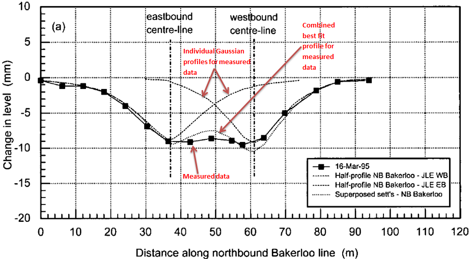
Figure 20 – Settlement troughs caused by excavation of JLE twin tunnels underneath the existing northbound Bakerloo line tunnel ^[7]

Figure 20 shows that the settlement at the intersection of the individual Gaussian profiles for the measured data is less than the settlement of the combined best fit profile in this same region. This indicates that there was an interaction effect between the two Gaussian profiles, meaning that that the two profiles are not independent of each other.

For JLE tunnelling at Waterloo underneath the existing northbound and southbound Northern line tunnels, Figure 21 shows that the combined best fit profile still has slightly greater settlements at the twin tunnel centreline, in comparison to the settlement at the intersection of the individual Gaussian profiles ^[7].

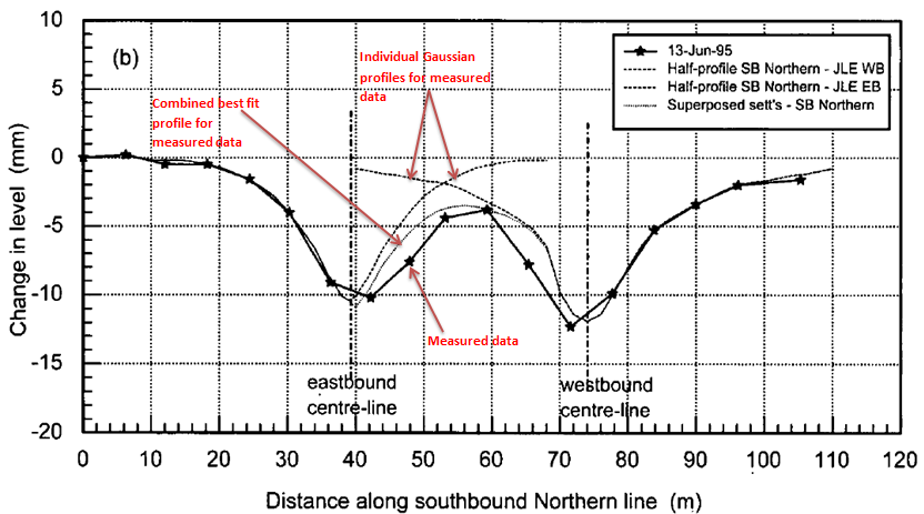
Figure 21 – Settlement troughs caused by excavation of JLE twin tunnels underneath existing southbound Northern line ^[7]

Standing and Selman in 2001 suggested several factors that may influence whether interaction between two settlement profiles occurs, including depth of the tunnel axis below the ground surface, axial separation of the tunnels, K values and relative position of the tunnel faces during construction ^[7].

Implications for future predictions

Equation 2 in this paper was used to fit curves to the settlement from levelling points, and the equation can be used to model surface settlement caused by parallel tunnels with different diameters, ground loss and trough width. Equation 2 also accounts for interaction between two Gaussian profiles using the S_AB term in the equation. This equation was successful in the curve fitting for the measured data along Arrays 1-3. Although the S_AB interaction term was equal to zero for Arrays 2 and 3, the equation still managed to model surface settlement at the centreline of the parallel tunnels that matched the measured data well (i.e. still managed to capture the interaction behaviour). The measured data therefore indicates that Equation 2 is an accurate function describing settlement caused by parallel tunnels. The JLE results also indicate that predictions for surface settlement due to parallel tunnels would be more accurate if the predictions account for interaction of the two settlement profiles.

Potential impact on buildings

The larger settlements observed at the centreline of parallel tunnels results in a settlement profile with a shallower gradient. Shallower gradients of settlement may result in less differential settlement of buildings located near the centreline of parallel tunnels, likely reducing the structural damage to buildings.

Comparison of eastbound and westbound tunnel results

Accounting for dewatering

To allow for the assessment of tunnel-induced settlement, surface settlement caused by dewatering (prior to excavation of tunnels) were deducted from surface settlements recorded for the levelling points on the dates presented in Appendix A.1. The maximum settlements attributed to dewatering were 6.0 mm (Array 1), 5.7 mm (Array 2) and 4.1 mm (Array 3), giving an average maximum dewatering settlement of 5.3 mm.

Since dewatering which occurred during the excavation of the SCL sections was not accounted for in the assessment of tunnel-induced settlement, it is possible that the volume losses presented in this paper are over-estimates.

Comparison of surface settlement and volume loss

The SCL Results section (and Appendices C.1, C.2 and C.3) of this paper provides EB and WB tunnel-induced surface settlement profile properties such as S_max, i, K and volume loss, for Arrays 1, 2 and 3 respectively.

The average volume loss due to excavation of the WB tunnel (considering Arrays 1-3) was 1.6%, and the average volume loss for the EB tunnel (considering Arrays 1 and 2 only) was also 1.6%. The SCL sections investigated indicate that overall, excavation of both tunnels had similar impacts on the ground movement.

The average K value for the WB tunnel (considering Arrays 1-3) was 0.58, while the average K value for the EB tunnel (considering Arrays 1 and 2 only) was 0.68. The EB tunnel is situated 5 m closer to the ground surface than the WB tunnel, causing the K values to be larger for the EB tunnel.

During the assessments of volume loss for Method 1, it is uncertain why for each tunnel on each array, the S_max value found by Solver and displayed in an Excel cell (S_max1) was not equal to the maximum settlement plotted by the best fit curve (S_max2). To be conservative, the greater volume losses were taken forward from Method 1 (as mentioned for each array in the SCL Results), before being compared to Method 2 results, allowing for a final volume loss to be chosen for each tunnel.

Potential impact of mixed ground conditions on WB tunnel results

Ignoring section G, the greatest measured volume loss was 2.1%, caused by excavation of the WB tunnel on Array 2. The empirical predictions of 0.5 for K and 1.5% for volume loss that were used are representative of typical values in London Clay based on case studies. However at Stepney Green, the bottom half of the WB tunnel is situated in the sandy Lambeth Group, and the top half is situated in London Clay. It has been reported that tunnelling in mixed face geological conditions can bring about higher volume losses ^[8]. This could explain why greater settlements were measured for the WB tunnel on Array 2, in comparison to the empirical predictions.

Comparison of volume loss caused by excavation of SCL sections with empirical prediction and O’Reilly and New values

When tunnelling in stiff fissured London Clay, volume losses generally lie in the range of 0.5-3.0% ^[9]. Excluding section G, the highest volume loss was 2.1%, which still fits within the range described by O’Reilly and New in 1982. The volume loss range described by O’Reilly and New were from a variety of tunnelling techniques, and a comparison of the Stepney Green results is provided later in this discussion against a specific SCL tunnelling case study.

The average volume loss caused by excavation of the investigated SCL sections (excluding section G on Array 3) was 1.6%. This shows that in general, tunnel excavation on site generated more surface settlement (and volume loss) in comparison to the empirical predictions. However, the average volume loss of 1.6% is very close to the empirical prediction of 1.5% that was used as a GRP input. The Crossrail empirical prediction of 1.5% volume loss due to SCL tunnelling at Stepney Green was based on previous experience and case studies for smaller SCL tunnels.

Comparison of K values from measured data with empirical prediction and O’Reilly and New values

O’Reilly and New proposed the following linear relationship between i and Z:

(3)

In Equation 3, O’Reilly and New proposed that the trough width factor, K, is equal to 0.5 for cohesive soils, but can range between 0.4 and 0.7 depending on the type of clay ^[9]. The K values stated by O’Reilly and New were based on the results of various case studies they had reviewed. The average K value (excluding section G) of 0.6 due to Stepney Green SCL tunnelling falls within the 0.4-0.7 range, supporting the proposal made by O’Reilly and New. Generally, the settlement curves for the measured data were wider than the predictions, resulting in a larger distance to the point of inflexion, hence leading to larger K values than predicted. However, the average measured K value of 0.6 is still close to the empirical prediction of 0.5.

Comparison of Stepney Green SCL volume loss and K results with JLE case study

Volume loss

Standing and Selman in 2001 presented volume loss values due to the 5.6 m outer diameter JLE tunnels constructed completely in London Clay in the Waterloo area, using SCL techniques. Volume loss values ranged from 0.5-1.1%, and the average volume loss was 0.86% ^[7].

The SCL tunnels at Stepney Green are far larger in size compared to the JLE running tunnels at Waterloo. The largest SCL section investigated is the EB tunnel (also completely in London Clay) on Array 2 which has an equivalent diameter of 14.374 m. Despite the EB tunnel on Array 2 being over two and a half times as large as the JLE running tunnels, the volume loss of 1.5% for the Stepney Green tunnel did not overwhelmingly exceed the average JLE volume loss at Waterloo.

Trough width factor, K

Standing and Selman also reported that K values for the JLE running tunnels at Waterloo ranged from 0.61-0.92, with an average K value of 0.75 ^[7]. The average K value for Stepney Green sections investigated in this report was 0.6, with a range of 0.51-0.72. The JLE case study indicates that it is not unusual to observe K values greater than 0.5 for SCL tunnels in London Clay.

Conclusions

Accounting for dewatering at the Stepney Green site seemed to be successful in isolating tunnel-induced settlement due to excavation of the SCL tunnels. Array 1 is a particularly good example of measured settlements along the entire length of the array being very close to the empirical settlement predictions, once dewatering was accounted for.

Excavation of SCL parallel tunnels at Stepney Green produced settlement profiles in the form of two merging Gaussian profiles. Equation 2 which accounted for interaction between two Gaussian profiles was successful in providing curve fits for the measured data, despite the interaction term being equal to zero for two arrays. The Stepney Green SCL surface monitoring results revealed greater settlements at the centreline of the parallel tunnels compared to the empirical estimates, which did not account for an interaction effect in the superposition of the two Gaussian profiles. The Stepney Green results and the case study mentioned in the discussion indicate that better predictions for settlements due to parallel tunnels can be achieved if predictions account for an interaction effect.

The Stepney Green data showed that the average volume loss due to excavation of the westbound tunnel was 1.6%, and the average volume loss due to excavation of the eastbound tunnel was also 1.6%. The results indicate that in terms of volume loss, construction of both SCL tunnels had the same overall impact on the ground surface at the Stepney Green site.

The average volume loss caused by SCL tunnelling at the Stepney Green site was 1.6%, and the empirical prediction was 1.5%. The Stepney Green SCL results show the accuracy of the volume loss prediction used in the empirical estimations. The average trough width factor, K, observed from measured data for the SCL sections was 0.6, and the prediction of K used in the empirical work was 0.5. This again shows good agreement with the empirical predictions for SCL tunnelling at the Stepney Green site.

The volume losses and K values observed from the large SCL tunnels at Stepney Green fall within the ranges described by O’Reilly and New in 1982 which were based on various tunnelling case studies. The Stepney Green results also compare well with the SCL tunnelling case study discussed in this paper. The results of this investigation show that the large SCL caverns at Stepney Green generate volume losses that do not overwhelmingly exceed volume losses of other SCL tunnels far smaller in size.

Acknowledgements

The author would like to acknowledge Crossrail, Dragados Sisk Joint Venture, Geocisa UK, Mott MacDonald, OTB Engineering and WJ Groundwater for the provision of many of the figures in this paper. The author would also like to thank Peter Rutty (Mott MacDonald), Dave Harris (Mott MacDonald) and Dr Rick Woods (University of Surrey) for their invaluable time.

References

[1] Harris, D., Davis, A., & Linde-Arias, E. (2014). Crossrail Sprayed Concrete Lining Depressurisation at Stepney Green Caverns. Crossrail Legacy Learning, [Online] Available at: <https://learninglegacy.crossrail.co.uk/documents/crossrail-sprayed-concrete-lining-depressurisation-at-stepney-green-caverns/ > [Accessed 20 May 2017]

[2] Harris, D., Davis, A., & Linde-Arias, E. (2014). Crossrail Sprayed Concrete Lining Depressurisation at Stepney Green Caverns (PowerPoint Presentation). Crossrail Limited.

[3] Crossrail Limited (2013). Construction of eastbound cavern at Stepney Green complete. [online] Available at: <http://www.crossrail.co.uk/news/articles/construction-of-eastbound-cavern-at-stepney-green-complete> [Accessed 20 May 2017]

[4] New, B.M. & O’Reilly, M.P. (1991). Tunnelling induced ground movements; predicting their magnitude and effects. Invited review paper to 4th International Conference on Ground Movements and Structures 1991, Pentech Press, pp. 671-697.

[5] Divall, S., Goodey, R.J. & Taylor, R.N. (2012). Ground movements generated by sequential twin-tunnelling in over-consolidated clay. Proceedings of the 2nd European

Conference on Physical Modelling in Geotechnics (Eurofuge 2012), Delft University

of Technology.

[6] Wang, J.G., Kong, S.L. & Leung, C.F. (2003). Twin tunnels-induced ground settlement in soft soils. Proceedings of the Sino-Japanese Symposium on Geotechnical Engineering 2003, Tsinghua University Press, pp. 241-244.

[7] Standing, J.R. & Selman, R. (2001). The response to tunnelling of existing

tunnels at Waterloo and Westminster. In: Burland, J.B., Standing, J.R. & Jardine, F.M., eds. 2001. Building Response to Tunnelling – Volume 2: Case Studies. 1st edn. London: Thomas Telford Publishing. pp.509-546.

[8] Mair, J.R. & Jardine, F.M. (2001). Tunnelling methods. In: Burland, J.B., Standing, J.R. & Jardine, F.M., eds. 2001. Building Response to Tunnelling – Volume 1: Projects and Methods. 1st edn. London: Thomas Telford Publishing. pp.127-134.

[9] O’Reilly, M.P. & New, B.M. (1982). Settlements above tunnels in the United Kingdom – their magnitude and prediction. Proceedings Tunnelling ’82 Symposium 1982, Institution of Mining and Metallurgy, pp. 173-181.

[10] McCallum, J. (2008). Ground Response Program User Guide. 5.0.4 edn.

[11] Attewell, P.B. & Woodman, J.P. (1982). Predicting the dynamics of ground settlement and its derivatives caused by tunnelling in soil. Ground Engineering, 15(8), pp.13-22, 36.

 

Appendices

Appendix A.1 – Summary of levelling points and dates used for investigation of SCL sections

Table 10

Array no.	Volume of excavated face, VF (m3/m)	Levelling points used in investigation (order of south to north)	Date of measurements used
1	VF for WB tunnel = 54.633 m3/m (equivalent diameter of 8.34 m)   VF for EB tunnel = 54.633 m3/m + 70%*(65.958 m3/m-54.633 m3/m) =  62.561 m3/m (equivalent diameter of 8.925 m)	LP072122, LP072121, LP072120, LP072119, LP072118, LP072117, LP072116, LP072115, LP072113, LP072112, LP072111, LP072110, LP072109, LP072106, LP072104, LP072103	28.1.14. All Stepney Green excavation and primary SCL works were completed by this date.
2	VF for WB tunnel = 70.790 m3/m + 90%*(120.013 m3/m-70.790 m3/m) = 115.091 m3/m (equivalent diameter of 12.105 m)   VF for EB tunnel = 120.013 m3/m + 70%*(180.387 m3/m-120.013 m3/m) = 162.275 m3/m (equivalent diameter of 14.374 m)	LP072504, LP072505, LP072506, LP072507, LP072508, LP072510, LP072511, LP072512, LP072515, LP072516, LP072519, LP072520, LP072522, LP072524, LP07009, LP07008, LP07007, LP07006, LP07005, LP07073	31.1.14. All Stepney Green excavation and primary SCL works were completed by this date.
3	VF for WB tunnel = 120.013 m3/m + 65%*(180.387 m3/m-120.013 m3/m) = 159.256 m3/m (equivalent diameter of 14.240 m)   VF for EB tunnel = 54.633 m3/m (equivalent diameter of 8.34 m)	LP072402, LP072405, LP072406, LP072407, LP072408, LP072409, LP072410, LP072411, LP072414, LP072415, LP072301, LP07078	31.1.14. All Stepney Green excavation and primary SCL works were completed by this date.

 

Appendix A.2 – Summary of levelling points and dates used for measuring dewatering induced settlement

Table 11

Array no.	Levelling points selected to investigate dewatering induced settlement	Date of measurements used
1	Same as in Appendix A.1	26.11.12. This date is before any excavation works occurred at Stepney Green.
2	Same as in Appendix A.1	21.11.12 for points LP2504 to LP07005, and 22.11.12 for point LP07073. These dates are before any excavation works occurred at Stepney Green. Surface settlement readings were not recorded for LP07073 on 21.1.12, so reading on 22.11.12 was used instead.
3	Same as in Appendix A.1	5.12.12 for points LP072402 to LP072301, and 6.12.12 for point LP07078. Surface settlement readings were not recorded for points LP072402 to LP072301 before 5.12.12, so this date was used. Surface settlement readings were not recorded for LP07078 on 5.12.12, so reading on 6.12.12 was used instead. Although excavation works for the tunnels commenced on 28.11.12, excavation was located far from this array, so it has been assumed that measured surface settlement on these dates will be purely due to dewatering.

 

Appendix B.1 – Additional information on arrays used in investigation

Table 12

Array no.	Assumed tunnel centreline locations	Axial separation, D (m)	Total cumulative distance along array (m)
1	WB centreline assumed to be 0.67 of the way between LP072119 and LP072118. EB centreline assumed to be at point LP072107.	43.421	71.518
2	WB centreline assumed to be midway between LP072509 and LP072510. EB centreline assumed to be at point LP07009.	52.564	113.084
3	WB centreline assumed to be midway between LP072408 and LP072409. EB centreline assumed to be 0.13 of the way between LP072301 and LP07078.	59.032	131.083

 

Appendix B.2 – Solver curve fitting procedure

Table 13

Step 3.1	Finding a mathematical function that would best fit the measured data.
Step 3.2	Entering the mathematical function in Excel, and using the function to find surface settlement at the same locations as the levelling points. Note that the surface settlements produced by the mathematical functions are termed S,Solver in this investigation.
Step 3.3	Creating a column that calculated the square of the difference between the measured surface settlement (S), and the surface settlement produced using the mathematical function, i.e. (S-S,Solver)2
Step 3.4	Calculating the sum of the square differences at the bottom of the column, i.e. Σ(S-S,Solver)2
Step 3.5	Use Solver to minimise the sum of the square differences by changing the variables that form the mathematical function. Note that when Solver minimises the sum of the square differences, at the same time it changes the values of S,Solver (i.e. the surface settlement produced by the mathematical function at each point changes). As a result, Solver can be used to find surface settlement defined by a mathematical function that is as close as possible to the measured data.
Step 3.6	Use the mathematical function to find surface settlement at locations between levelling points and outside the array of levelling points (at 1m intervals), so that a fully developed best fit settlement profile can be produced.

 

Appendix B.3 – Method 1 of assessing volume loss

Equation 4 can be used to find the volume of settled material per metre, V_s (m³/m):

(4)

In this equation, i is the distance from the tunnel centreline to the point of inflexion on the curve and S_max is the maximum settlement above a tunnel ^[9].

As shown in Equation 2 earlier in this paper, the mathematical function representing the settlement caused by parallel tunnels includes variables such as i and S_max for each tunnel. Solver finds values for the variables i and S_max for each tunnel which give an overall best fit curve for the levelling point data along an array.

Method 1 of assessing volume loss involves the calculation of V_s for each tunnel (Equation 4), using Solver values of i_A and S_max,A to calculate V_S,A, and using Solver values of i_B and S_max,B to calculate V_S,B. The volume loss of tunnel ‘A’ and tunnel ‘B’ can be found by dividing the V_S value by the excavated volume of each tunnel face, V_F (see Appendix A.1 for V_F values).

During the assessments, it was found that for each tunnel on each array, the S_max value determined by Solver and displayed in the Excel cell was not equal to the maximum settlement plotted by the best fit curve (reason unknown). Therefore for each tunnel, Method 1 has two S_max values (and hence two volume loss values):

• S_max1: the maximum settlement above the tunnel determined by Solver and the value is located in an Excel cell.
• S_max2: the maximum settlement above the tunnel, which is taken directly from the best fit curve.

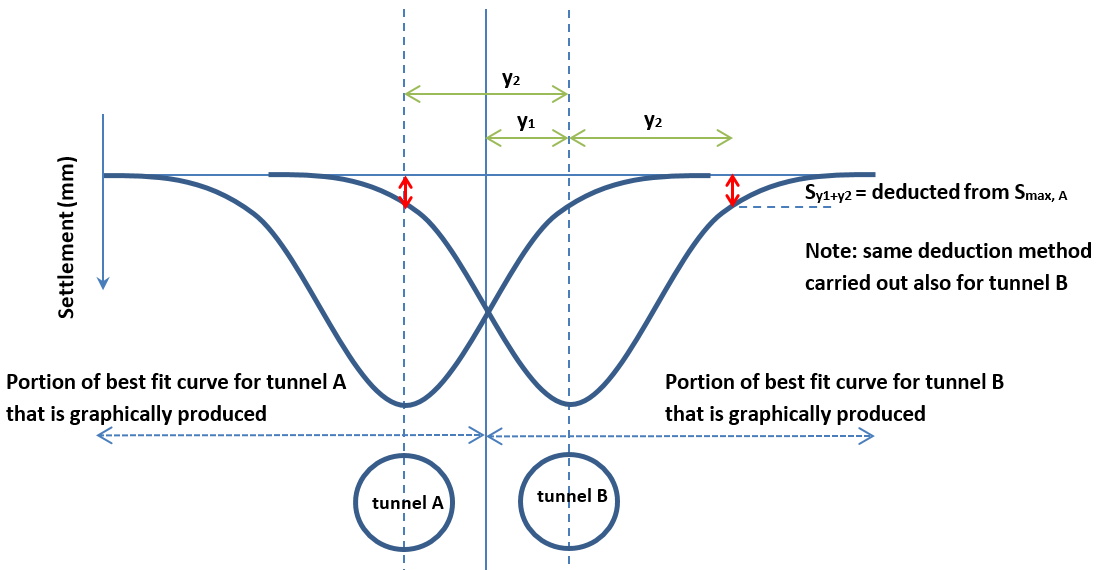
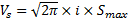
Before volume loss is calculated for each tunnel, Method 1 also attempts to reduce the maximum settlement caused by each tunnel, due to the potential for one settlement curve to influence the other (see Figure 22). For example, the numbered points below summarise the process of deducting the maximum settlement above tunnel A due to the influence of the tunnel B settlement curve (i.e. if the settlement curve of tunnel B crosses the plane of the maximum settlement above tunnel A):

1. Finding the distance between the centreline of tunnel B and the position (along the best fit curve) of the maximum settlement above tunnel A (y₂).
2. Finding the settlement on the best fit curve at position y₁ + y₂ (nearest m used) above tunnel B (S_y1+y2).
3. Deducting S_y1+y2 from the maximum settlement above tunnel A (S_{max, A}). This is based on the assumption that the best fit curve produced above tunnel B is symmetrical, since the full Gaussian curve for tunnel B is not graphically produced.
4. Repeat the same process to deduct the maximum settlement above tunnel B.

Note that in some instances, S_y1+y2 is equal to zero settlement (e.g. if y₁+y₂ is located beyond a tunnel’s best fit curve).

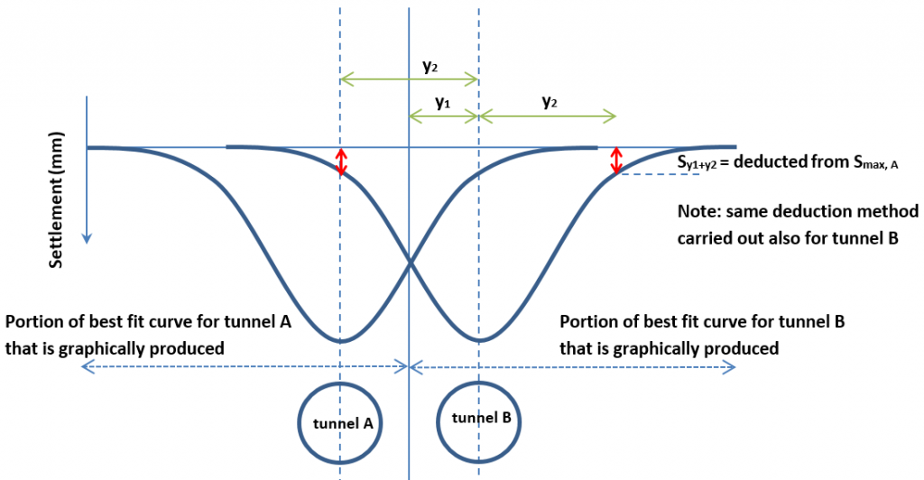
Figure 22 – Deduction of maximum settlement above each tunnel for Method 1 volume loss calculations

Appendix B.4 – Method 2 of assessing volume loss

The process for calculating volume loss in Method 2 is summarised by Figure 23 and the numbered points below (in the example below, excavation for tunnel B is before tunnel A excavation):

1. Determining the volume of settled material per m underneath the S,_Solver points for the tunnel B half curve using the trapezium rule (V_{S, 0.5 trap B}). The half curve is between the maximum settlement on the best fit curve above tunnel B and the last S,_Solver point on the curve.
2. Determining the volume of settled material per m for the tunnel B full curve (V_{S, trap B}). This is based on the assumption that the best fit curve produced above tunnel B is symmetrical, since the full Gaussian curve for tunnel B is not graphically produced (i.e. V_{S, 0.5 trap B} is simply doubled). The volume loss for tunnel B can then be calculated.
3. Determining the volume of settled material per m underneath the S_,Solver points for the entire best fit curve using the trapezium rule (V_{S, trap}).
4. Determining the volume of settled material per m for due to tunnel A (V_{S, trap A}) by subtracting V_{S, trap B} from V_{S, trap}. The volume loss for tunnel A can then be calculated.

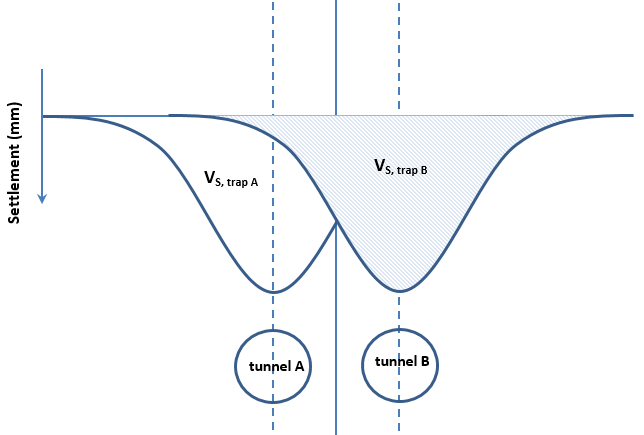
Figure 23 – Method 2 volume loss calculation diagram

Appendix B.5 – GRP inputs and vertical surface settlement equation

For analysing tunnels, the program requires the input of tunnel properties, and GRP has the ability to analyse ground movements due to any number of tunnels. Inputs for a tunnel include the x y coordinates at either end of the tunnel (m), the depth to the tunnel axis level at either end of the tunnel Z (m), the volume loss V_L (%), the trough width factor K, the diameter of the tunnel D (m) and the ribbon width (W) which can be set to zero for point sink analysis ^[10]. Note that GRP will use interpolation of the properties just listed in order to find values in between the tunnel ends. Also note that GRP assumes that all tunnels are circular, however as can be seen in Figures 6-8, the SCL sections at Stepney Green are not completely circular.

GRP calculates vertical settlement using the equation below:

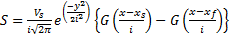(5)

In Equation 5: S is vertical settlement; V_s is the volume of settled material; i is the distance from the tunnel centreline to the point of inflexion on the settlement curve; y is the transverse distance from the tunnel centreline; x is the position along the tunnel parallel to its axis; x_s is the position at the start of the tunnel; x_f is the position at the end of the tunnel and G is the normal cumulative distribution function ^[10]. This equation was presented by Attewell and Woodman in 1982 in the publication entitled “Predicting the dynamics of ground settlement and its derivatives caused by tunnelling in soil” ^[11].

Appendix C.1 – Full results tables for Array 1

Table 14 – Method 1 results for WB tunnel

Transverse distance from the centreline of the parallel tunnels to centreline of EB tunnel, y1 (m)	21.711
Transverse distance from the centreline of the EB tunnel to position of Smax, WB, y2 (m)	41.202
y1 + y2 (m)	62.913
Settlement on best fit curve at position y1 + y2 above the EB tunnel, Sy1+y2 (m)	0.0000
Distance from WB centreline to point of inflexion on curve, iWB (m)	15.366
VF, WB (m3/m)	54.633
Smax1, WB (m)	0.0164
Smax1, WB – Sy1+y2 (m)	0.0164
Volume of settled material per m due to WB tunnel using Smax1, WB – Sy1+y2 value, VS1, WB (m3/m)	0.632
VL1, WB (m3/m)	1.157
Smax2, WB (m)	0.0150
Smax2, WB – Sy1+y2 (m)	0.0150
Volume of settled material per m due to WB tunnel using Smax2, WB – Sy1+y2 value, VS2, WB (m3/m)	0.578
VL2, WB (m3/m)	1.058
Ground level for WB tunnel (mATd)	110.000
WB tunnel axis depth (mATd)	80.000
WB tunnel axis depth below ground level, ZWB (m)	30.000
K for WB tunnel, KWB	0.512

 

Table 15 – Method 1 results for EB tunnel

Transverse distance from the centreline of the parallel tunnels to centreline of WB tunnel (y1, m)	-21.711
Transverse distance from the centreline of the WB tunnel to position of Smax, EB (y2, m)	-42.711
y1 + y2 (m)	-64.422
Settlement on best fit curve at position y1 + y2 above the WB tunnel, Sy1+y2 (m)	0.0000
Distance from EB centreline to point of inflexion on curve, iEB (m)	15.780
VF, EB (m3/m)	62.561
Smax1, EB (m)	0.0268
Smax1, EB – Sy1+y2 (m)	0.0268
Volume of settled material per m due to EB tunnel using Smax1, EB – Sy1+y2 value, VS1, EB (m3/m)	1.060
VL1, EB (m3/m)	1.694
Smax2, EB (m)	0.0250
Smax2, EB – Sy1+y2 (m)	0.0250
Volume of settled material per m due to WB tunnel using Smax2, EB – Sy1+y2 value, VS2, EB (m3/m)	0.989
VL2, EB (m3/m)	1.581
Ground level for EB tunnel (mATd)	110.000
EB tunnel axis depth (mATd)	85.000
EB tunnel axis depth below ground level, ZEB (m)	25.000
K for EB tunnel, KEB	0.631

 

Table 16 – Method 2 results for both tunnels

Volume of settled material per m underneath the S,Solver points for EB tunnel half curve using the trapezium rule, VS, 0.5 trap EB (m3/m)	0.462
Volume of settled material per m for EB tunnel half curve doubled, VS, trap EB (m3/m)	0.924
VF, EB (m3/m)	62.561
VL, EB (m3/m)	1.477
Volume of settled material per m underneath the S,Solver points for entire curve using the trapezium rule, VS, trap (m3/m)	1.435
VS, trap WB (m3/m)	0.511
VF, WB (m3/m)	54.633
VL, WB (m3/m)	0.935

 

Appendix C.2 – Full results tables for Array 2

Table 17 – Method 1 results for WB tunnel

Transverse distance from the centreline of the parallel tunnels to centreline of EB tunnel, y1 (m)	26.282
Transverse distance from the centreline of the EB tunnel to position of Smax, WB, y2 (m)	51.398
y1 + y2 (m)	77.680
Settlement on best fit curve at position y1 + y2 above the EB tunnel, Sy1+y2 (m)	0.0008
Distance from WB centreline to point of inflexion on curve, iWB (m)	20.223
VF, WB (m3/m)	115.091
Smax1, WB (m)	0.0485
Smax1, WB – Sy1+y2 (m)	0.0477
Volume of settled material per m due to WB tunnel using Smax1, WB – Sy1+y2 value, VS1, WB (m3/m)	2.418
VL1, WB (m3/m)	2.101
Smax2, WB (m)	0.0493
Smax2, WB – Sy1+y2 (m)	0.0485
Volume of settled material per m due to WB tunnel using Smax2, WB – Sy1+y2 value, VS2, WB (m3/m)	2.459
VL2, WB (m3/m)	2.137
Ground level for WB tunnel (mATd)	111.000
WB tunnel axis depth (mATd)	80.000
WB tunnel axis depth below ground level, ZWB (m)	31.000
K for WB tunnel, KWB	0.652

 

Table 18 – Method 1 results for EB tunnel

Transverse distance from the centreline of the parallel tunnels to centreline of WB tunnel (y1, m)	-26.282
Transverse distance from the centreline of the WB tunnel to position of Smax, EB (y2, m)	-51.282
y1 + y2 (m)	-77.564
Settlement on best fit curve at position y1 + y2 above the WB tunnel, Sy1+y2 (m)	0.0018
Distance from EB centreline to point of inflexion on curve, iEB (m)	17.878
VF, EB (m3/m)	162.275
Smax1, EB (m)	0.0537
Smax1, EB – Sy1+y2 (m)	0.0519
Volume of settled material per m due to EB tunnel using Smax1, EB – Sy1+y2 value, VS1, EB (m3/m)	2.326
VL1, EB (m3/m)	1.433
Smax2, EB (m)	0.0555
Smax2, EB – Sy1+y2 (m)	0.0537
Volume of settled material per m due to WB tunnel using Smax2, EB – Sy1+y2 value, VS2, EB (m3/m)	2.406
VL2, EB (m3/m)	1.483
Ground level for EB tunnel (mATd)	110.000
EB tunnel axis depth (mATd)	85.000
EB tunnel axis depth below ground level, ZEB (m)	25.000
K for EB tunnel, KEB	0.715

  

Table 19 – Method 2 results for both tunnels

Volume of settled material per m underneath the S,Solver points for EB tunnel half curve using the trapezium rule, VS, 0.5 trap EB (m3/m)	1.286
Volume of settled material per m for EB tunnel half curve doubled, VS, trap EB (m3/m)	2.572
VF, EB (m3/m)	162.275
VL, EB (m3/m)	1.585
Volume of settled material per m underneath the S,Solver points for entire curve using the trapezium rule, VS, trap (m3/m)	4.866
VS, trap WB (m3/m)	2.294
VF, WB (m3/m)	115.091
VL, WB (m3/m)	1.993

 

Appendix C.3 – Full results tables for Array 3

Table 20 – Method 1 results for WB tunnel

Transverse distance from the centreline of the parallel tunnels to centreline of EB tunnel, y1 (m)	29.516
Transverse distance from the centreline of the EB tunnel to position of Smax, WB, y2 (m)	57.516
y1 + y2 (m)	87.032
Settlement on best fit curve at position y1 + y2 above the EB tunnel, Sy1+y2 (m)	0.0021
Distance from WB centreline to point of inflexion on curve, iWB (m)	18.140
VF, WB (m3/m)	159.256
Smax1, WB (m)	0.0483
Smax1, WB – Sy1+y2 (m)	0.0462
Volume of settled material per m due to WB tunnel using Smax1, WB – Sy1+y2 value, VS1, WB (m3/m)	2.101
VL1, WB (m3/m)	1.319
Smax2, WB (m)	0.0502
Smax2, WB – Sy1+y2 (m)	0.0481
Volume of settled material per mdue to WB tunnel using Smax2, WB – Sy1+y2 value, VS2, WB (m3/m)	2.187
VL2, WB (m3/m)	1.373
Ground level for WB tunnel (mATd)	111.500
WB tunnel axis depth (mATd)	80.000
WB tunnel axis depth below ground level, ZWB (m)	31.500
K for WB tunnel, KWB	0.576

 

Table 21 – Method 1 results for EB tunnel

Transverse distance from the centreline of the parallel tunnels to centreline of WB tunnel (y1, m)	-29.516
Transverse distance from the centreline of the WB tunnel to position of Smax, EB (y2, m)	-58.516
y1 + y2 (m)	-88.032
Settlement on best fit curve at position y1 + y2 above the WB tunnel, Sy1+y2 (m)	0.0000
Distance from EB centreline to point of inflexion on curve, iEB (m)	23.708
VF, EB (m3/m)	54.633
Smax1, EB (m)	0.0395
Smax1, EB – Sy1+y2 (m)	0.0395
Volume of settled material per m due to EB tunnel using Smax1, EB – Sy1+y2 value, VS1, EB (m3/m)	2.347
VL1, EB (m3/m)	4.296
Smax2, EB (m)	0.0397
Smax2, EB – Sy1+y2 (m)	0.0397
Volume of settled material per m due to WB tunnel using Smax2, EB – Sy1+y2 value, VS2, EB (m3/m)	2.359
VL2, EB (m3/m)	4.318
Ground level for EB tunnel (mATd)	110.000
EB tunnel axis depth (mATd)	85.000
EB tunnel axis depth below ground level, ZEB (m)	25.000
K for EB tunnel, KEB	0.948

 

Table 22 – Method 2 results for both tunnels

Volume of settled material per m underneath the S,Solver points for EB tunnel half curve using the trapezium rule, VS, 0.5 trap EB (m3/m)	1.188
Volume of settled material per m for EB tunnel half curve doubled, VS, trap EB (m3/m)	2.376
VF, EB (m3/m)	54.633
VL, EB (m3/m)	4.349
Volume of settled material per m underneath the S,Solver points for entire curve using the trapezium rule, VS, trap (m3/m)	4.532
VS, trap WB (m3/m)	2.156
VF, WB (m3/m)	159.256
VL, WB (m3/m)	1.354