1. Introduction

In order to assess potential movements and the risk to the assets during and after construction, a monitoring system with suitable levels of accuracy, repeatability and frequency is required to provide construction teams with up to date information on which to base construction decisions. The optical system (Robotic Total Stations (RTS) and 3D Prisms) has been widely used on Crossrail for this purpose and this shall be the main focus of this paper.

As part of the risk assessment procedure prior to starting construction it is necessary to carry out damage assessments for all foundations and structures within the zone of influence (ZOI) of a potential construction. These assessments provide absolute deformation parameters for each asset such as the maximum tensile building strain for different building lengths in each hogging and sagging zone, the maximum bending and shearing tensile strains for short and long buildings and the bending and horizontal strain components for short and long buildings. Generally, these parameters are compared to the predicted volume losses and a risk-based approach to damage assessment is adopted with triggers determined accordingly.

The problems arise when the reality doesn’t fit the predictions, when the real data shows that although there might not be construction activity, there is structural movement due to other factors that were never considered, or even that the real movement is masked by what could be considered as noise, being in reality the structures natural behaviour before the construction activity started.

The intention of this paper is to encourage the reader to consider the stated accuracies of different monitoring systems and challenges them to question the need for and validity of such high precision when there are so many factors contributing to the observed movements. The paper also aims to provide more realistic and applicable accuracies and suggests how new technologies can help in large monitoring schemes.

2. Where and what to monitor

The Crossrail Civil Engineering Design Standard (CEDS) Part 8 (Crossrail, 2010) describes a risk-based approach to the assessment of existing structures and mitigation design whereby all assets lying within the Zone of Influence (ZOI) of the works are identified, assessed, monitored and closed out.

The buildings within the 10mm settlement contour are categorised by their building damage assessment parameters (Figure 1) to obtain the building damage classification (Table 1) after (Mair, Taylor, & Bracegirdle, 1993).

Regardless of the damage classification we assume that the structures within the ZOI will behave in the same way. The triggers that are set up afterwards for the monitoring are based on this prediction, not on the specific shape, construction, or position of the structure vs the excavation. Most commonly the triggers that will be set up to monitor the assets will be directly linked to the reaction (in terms of settlement or tilt) of the structure towards the construction activity, in very few occasions to directly measure the stress or tensile strain.

Figure 1: Building damage assessment parameters, (Devriendt, 2005)

Table 1: Building damage classification, (Mair, Taylor, & Burland, 1996)

This means that in general design predictions are based on broad assumptions (i.e. Greenfield conditions, building modelled using beam theory, settlement empirically matched to a Gaussian curve, etc.) and a limited set of parameters. Triggers are then based on design predictions and ignore environmental effects or instrumentation system accuracies.

3. Monitoring techniques and their repeatability

The values recorded from a monitoring system will consist of the seasonal variations affecting the ground and the asset together with the construction event affecting the same plus the accuracy and precision of the system itself. In order to effectively analyse data from the monitoring systems it is important to understand the definition of some terms when reporting measurements, assessing instrument performance, and estimating the degree of uncertainty in the methods (Standing, Withers, & Nyren, 2001). As they did in their book, we will quote the ones used by Dunnicliff (Dunnicliff, 1993).

Resolution is the smallest division readable or measurable on the instrument. Interpolation by eye between divisions generally does not improve the resolution, as the estimation is subjective and operator dependent.

Accuracy is the degree of correctness of a measurement, or the nearest of a measurement to the true quantity. The accuracy of a measurement depends on the accuracy of each component of the monitoring system. It is generally evaluated during instrument calibration, where a known value and the measured value are compared. Accuracy is expressed as ±x units, meaning that the measurement is within x units of the true value.

Precision is the reproducibility and repeatability of a measurement, or the nearness of each of a number of measurements to the arithmetic mean. Is also expressed in ±x units, meaning that the measurement is within x units of the mean measured value and is often assessed statistically with a degree of confidence associated with the statistical distribution.

Noise describes the random measurement variation by external factors. Excessive noise results in lack of precision and accuracy, and may conceal small real changes in the measured parameter.

Repeatability is the variation in measurements taken by a single person or instrument on the same item, under the same conditions, and in a short period of time. A less-than-perfect test–retest reliability causes test–retest variability. Such variability can be caused by, for example, intra-individual variability and intra-observer variability. A measurement may be said to be repeatable when this variation is smaller than a pre-determined acceptance criteria

The above definition of accuracy refers to the measurements. But when considering the accuracy of the monitoring system, this aspect is not as straightforward. It needs to be clarified that the overall accuracy or precision of the monitoring system can vary between different installations and instrumentation used. It should always be assessed individually on the case by case basis. For example the accuracy of the RTS network is a function of several factors such as:

All these factors can contribute to overall accuracy of the monitoring system. Thus it is a sensible practice to assess the network accuracy during the design phase by using least squares adjustment simulation. It will ensure that the system has sufficient sensitivity to detect movements and in case the results are not satisfactory, appropriate improvements to the network performance could be applied.  The same applies to manual monitoring and any other monitoring system like water levelling cells, inclinometers, extensometers, etc. that are read as part of a system. In manual levelling every circuit of levelling points (BRE sockets, track levelling marks, etc.), will have a different repeatability which will have to be defined at every case, depending on the constraints (length of the transect, number of stations, distance between stations, same surveyor and assistant taking the readings, taking them at the same time of the day and other number of factors that could introduce noise in the daily readings).

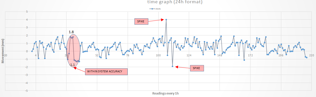
As mentioned above, one of the most crucial roles in assessing reliability of monitoring system is its precision and repeatability. From our experience, the interpretation of this factor can cause some confusion, so to clarify this concept we will use an example of the vertical movement of a prism as illustrated in Figure 2.

Figure 2 shows the vertical movement of a prism over time drawn with a “thin pen”. If we assume the system accuracy/repeatability is expected within ±1.5 mm band and the difference from two consecutive readings is 2.9mm it should not be concluded that the movement occurred, unless the following readings confirm formation of a trend, moreover this difference is within system accuracy. Another event frequently noticeable in the data and often leading to misinterpretation are spikes. A spike is a drastic change of reading usually followed by the reading similar to the one before the event occurred. In other words, it is just an error, which could be caused by several possible factors. This anomaly should be ignored and not regarded as a movement.  Spikes can be caused by several factors, such us an obstruction in one or more of the reference prisms in one cycle, an erroneous reading in one specific prism in one specific cycle, etc.

Figure 2: Vertical movement of a prism read through an RTS network over time drawn with a “thin pen”.

In our opinion the confusion in using a thinner pen to draw and then interpret the data could and should be avoided. If the daily average or median was reported instead of (or additionally to) the hourly median, as shown in Figure 5, much more meaningful conclusions could be drawn from the data. As the main subject in this paper is pointing out that using a thicker pen and analysing the trends could be more beneficial in drawing any conclusions than all the set of available data.

As shown in Figure 3, anything within the green band (±1.5 mm roughly) should be deemed acceptable, since it’s inside of the system’s monitoring accuracy, and that band does not show any significant movement over that specific period of time.

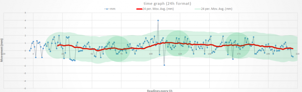
Figure 3: Vertical movement of a prism read through an RTS network over time drawn with a “thick pen”.

One of the most extensively used techniques in deformation current monitoring projects is the RTS network solution, or “optical system”. Because of its high repeatability and precision, it represents a good example of a monitoring technique capable of detecting small scale movements, the overall results are precise to the point, that even thermic fluctuations are recordable in the data. Whether these fluctuations are totally inherent to the structure, or they come from the system is irrelevant in this discussion, the fact is that thermic influence is clearly detectable and recordable (Figure 3), regardless of any construction activity taking place. With enough monitoring data there will be other seasonal behaviours that are as well visible to a keen eye.

These variations can move between fractions of a millimetre to couple of millimetres (although in extreme conditions it could be several more >10 mm), and since they are embedded in the monitoring system through sensors installed on the structures, they should be ignored and considered just as a noise. However in reality, these thermal fluctuations are often misinterpreted as a movement coming from construction activity or they can lead to loss of confidence in quality of monitoring system. Therefore the proposed approach of using a ‘thicker pen’ would be a worthwhile practice. Figure 4 to Figure 7 are further illustrations of this point.

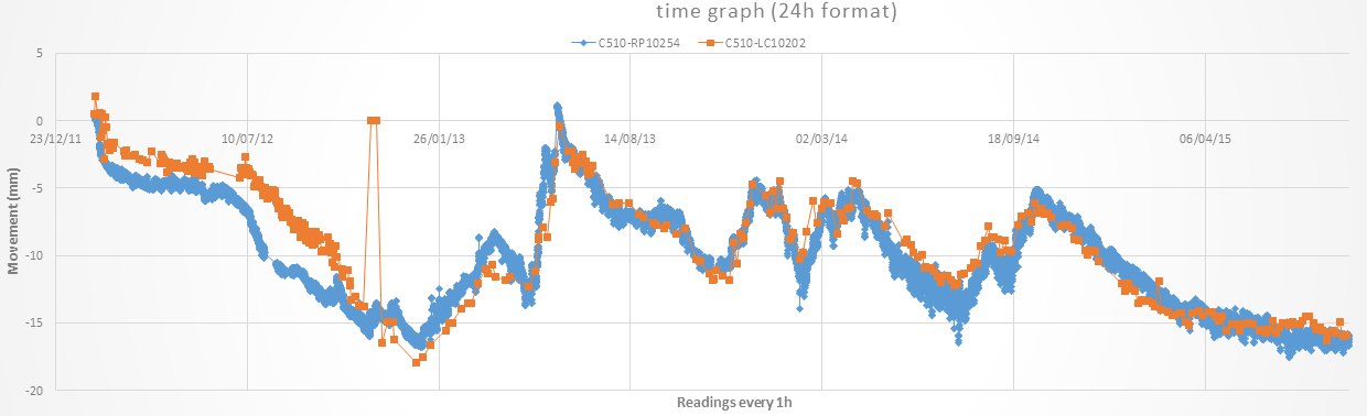
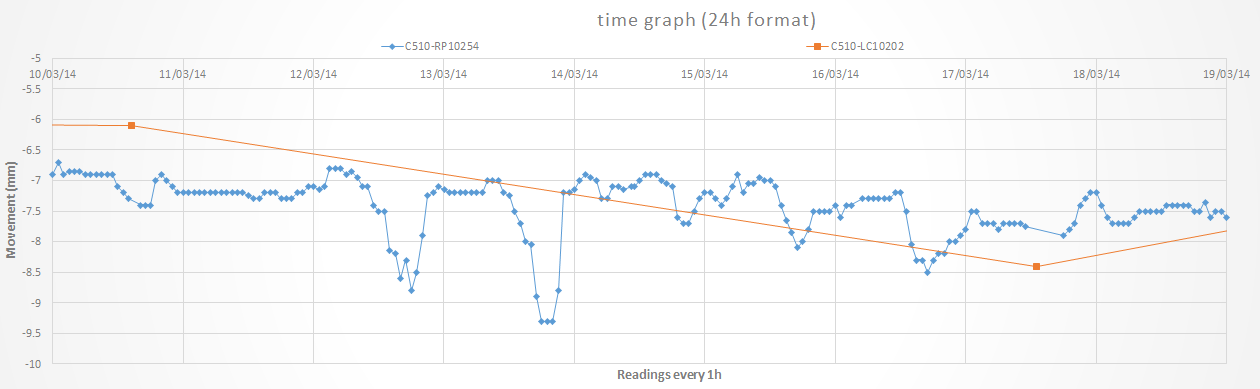
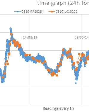
Figure 4: Total history of vertical movement over time from a prism (blue) and a barcode levelling bar (red)

Figure 4 shows the recorded behaviour of an automatically read prism by a networked RTS system (C510-RP10254) and a manually read barcode levelling bar (C510-LC10202), both installed on the same Victorian stone construction building but at different heights. Apart from some discrepancies, the behaviour of both of them over the monitored period of almost 5 years is quite comparable, and one would say that both systems were successful in recording the general movement. The large and rapid episodes of heave are linked to compensation grouting activity.

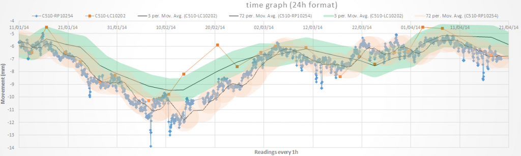
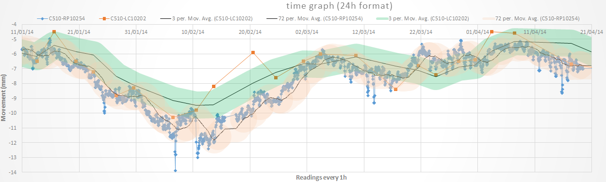
Figure 5: 3 months of vertical movement over time from a prism (blue) and a barcode levelling bar (red) with moving average trend lines

Figure 5 shows the same two sensors over a 3 month period with the addition of “thicker pen” trend lines based on a moving average. Although they both are still quite comparable now due to the shorter period, and the smaller scale we can start seeing some irregularities in both system, the automatic shows variations along the way, some of them quite out of the average, and the manual data looks more jumpy from one reading to the other, as well with some readings off the average. Highlighted in pale green and orange we can see what could be the expected monitoring accuracy as define previously, everything in within those areas should be considered as correct technically speaking, and according to a good practice. Over all one would say that the data still looks fine.

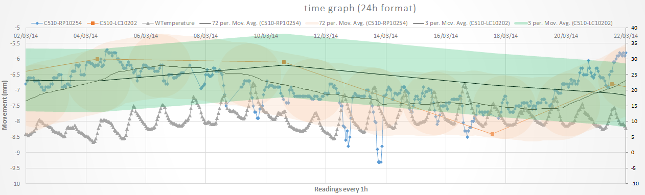
Figure 6: 3 weeks of vertical movement (mm) over time from a prism (blue) and a barcode levelling bar (red) with moving average trend lines and temperature (⁰C).

Figure 6 shows the same instruments over a 3 week period with the addition of temperature. The daily fluctuations and the jumps from one reading to the following one in the manual are even more apparent. Once more the shaded areas are highlighting what should be considered as normal in within their systems monitoring accuracy. Technical people with little experience in monitoring could potentially start complaining about the quality of the data. When looked at more closely it can be seen that there is a really good correlation between the data variations and the temperature ones, which means that the data variations are directly linked to the temperature. How to correct this noise due to temperature or how directly correlated to it is it, it’s not part of this paper.

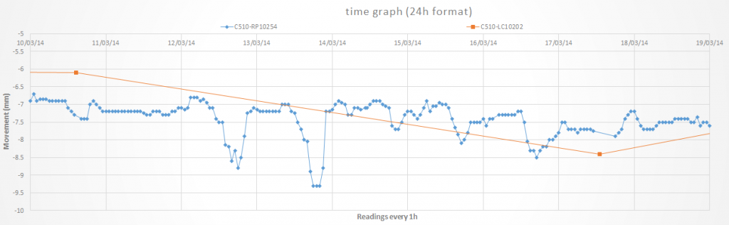
Figure 7: 1 week of vertical movement over time from a prism (blue) and a barcode levelling bar (red)

Figure 7 is the same data but limited to 1 week and is an example of what is often presented to at monitoring meetings with the stakeholders who can have limited experience of monitoring and how to interpret the readings. From this graph to the previous one the systems that suffers more is the prism due to its constant fluctuation. In taking this graph at face value one could be forgiven for concluding that the prism is unreliable and the barcode is showing a settlement of 2.5mm however, the reality is that the whole movement is within the monitoring accuracy of both systems and the asset is most likely stable.

It would appear then that both systems are far off what most technical specifications and academic papers (Standing, Withers, & Nyren, 2001) expect for precise levelling and automatic monitoring, see Table 2. It is all too common to mistake instrument accuracy and precision to what can be achieved when using those instruments in field conditions in a monitoring system.

Table 2: Examples of the best accuracies achieved for the various monitoring techniques (Standing, Withers, & Nyren, 2001)

In our experience we often come across the opinion, that the instruments with highest specification would provide the best results. But as we pointed out on several occasion in the paper, the factors introducing noise/error in to the systems reading will be occurring regardless which instrument is used. What makes a remarkable difference in terms of getting a good quality and repeatable data is processing or post-processing. This aspect is often ignored in the monitoring specifications under the umbrella of engaging a knowledgeable contractor that will be following the industry standards to get readings.  The only problem is – there are no accepted standards for most part of the I&M systems. Having said this, we still need to remember that even if the accuracies from the devices technical specifications were achievable on site, that accuracy and resolution would be two or more orders smaller than the expected movement in a normal construction environment, which doesn’t bring any significant benefit and justification by the project needs.

Moreover, the sub-millimetre accuracies stated are not necessary and add to the confusion during interpretation. Table 3 lists what the authors believe are more appropriate technical characteristics of monitoring systems discussed in this paper. As can be seen, although it is possible to get better resolutions with the digital equipment, we consider that anything below 0.1 mm in the normal construction environment is not really worth displaying, especially if the systems repeatability is worst that (as it is in all the examples provided).

The displayed repeatability values in Table 3 are based more on empirical observations from experience acquired on many projects including the largest monitoring scheme to date at Crossrail, although many could be explain applying levelling (surveying) basic error theories, but it was not the main objective of the paper. The factors affecting these parameters are difficult to quantify and will vary greatly depending on the site and office (processing) constraints (Gonzalez Marti, Brzeski, & Sanchez Barruetabena, 2016).

Table 3: Technical specification vs realistic on site accuracies achievable for selected monitoring systems.

4. Natural behaviour of structures and ground

The total observed displacement of the surface structure contents the deformation due to the external event and the deformation due to environmental factors and can be expressed by the following formula (Lian, 2015).

Equation 1: Total observed movement (Lian, 2015)

Where M_observed is the total movement, M_{external event} is the displacement from external event, such as tunnel excavation; M _thermal is the displacement due to thermal change; ε is the other influences in the observed value. It should be noted that with the exception of InSAR, all the movements recorded by the monitoring systems in table 4 are relative to their references. InSAR would be the only system providing real absolute movements making it an ideal tool for determining local trends.

Buildings will naturally move throughout the year, normally in a seasonal manner. This could be as a result of many factors pertaining to the structure itself or the ground in which it is founded. The purpose of this article is not to evaluate the reasons behind these movement trends but to raise awareness of these natural behaviours before, during, and after monitoring campaigns.

Seasonal events such as episodes of rainfall (or lack of them) can lead to structure and/or foundation damage. The UK the association of British insurers has estimated that the average cost of shrink-swell behaviour related subsidence stands at over £400 million a year (Jones & Jefferson, 2012).

In the context of infrastructure construction in urban environment, activities such as dewatering, decompression due to load removal or new or increased water influx can have an influence as well as the seasonal patterns of the soil. This is relevant in the context of the RTS networks, where optical properties such as percentage of visibility or standard deviation in readings from a prism over a 72h period are given a higher relevance during deployment. Buildings out of the ZOI used as reference can experience additional heave/settlement which can have an effect on the general behaviour of the network if unevenly spread over long monitoring periods. Figure 8 shows an example of such behaviour for a reference prism installed on a building outside of the ZOI. The readings clearly correlate with the seasonal trends (especially with distance readings) over the 2-years period of time and this natural behaviour needs to be taken into account when analysing the data.

Since it can be difficult to differentiate between regular seasonal movement and genuine movement, it is important to have a monitoring baseline period to determine the natural movement of the area. Satellite monitoring techniques such as InSAR can give a reasonable idea of the behaviour to be expected on a regional scale from buildings /structures without the need for installing and maintaining expensive monitoring systems.

 
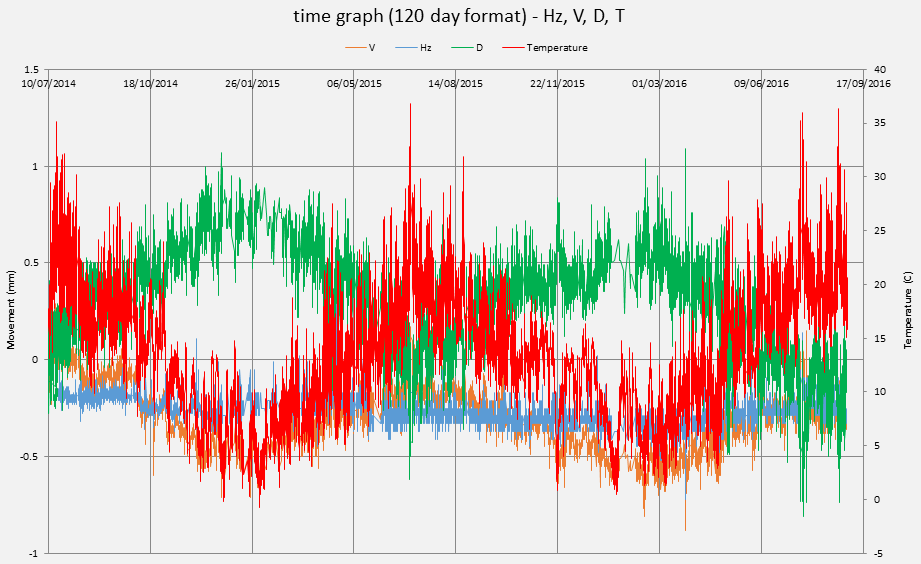
Figure 8: Seasonal trends detectable on horizontal, vertical angles and distances.

Figure 9 shows four areas where the local seasonal patterns are visible in InSAR data collected by Crossrail in areas well outside the ZOI of the works. Areas of relative proximity (such as Bond Street and Tottenham Court Road or Farringdon and Barbican to Moorgate) share common traits even though they are not exactly the same. The same episodes of settlement/heave repeat in the areas affected by the CRL works but can be masked with genuine movement.

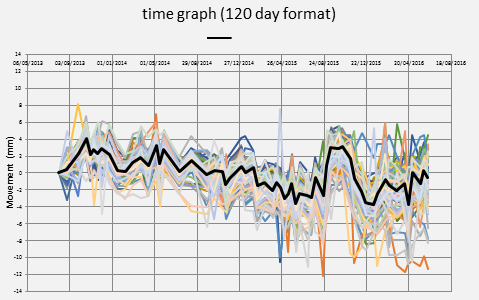
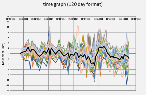
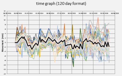
Figure 9: Seasonal patterns observed in InSAR data at various Crossrail Sites.

As a natural extension to these observations, if the satellite monitoring data is treated under the same principle of a total station or levelling network, stable areas outside of the works influence could be used to post-process readings in order to eliminate the local patterns or signatures converting the data into a relative dataset that could be compared with the conventional monitoring. Figure 10 illustrates this process by showing data from Barbican with the areas seasonal signature and then the same data with the affect removed.

The stability shown on the processed InSAR data demonstrates that it is feasible to use this approach when observing trends in the ZOI. Figure 11 shows “corrected” InSAR data over a three 3 year period at Bond Street demonstrating stability over long periods whilst keeping a good repeatability and a good correlation with more conventional forms of monitoring. This highlights the importance of using an appropriate timescale when analysing data and not just relying on the current values.

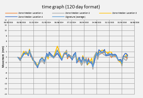
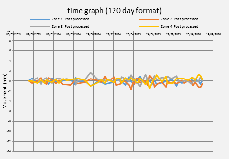
Figure 10: Overlapped seasonal patterns observed in InSAR data and outcome of the extraction of the average outcome proving stable behaviour at nearby the Barbican Centre.

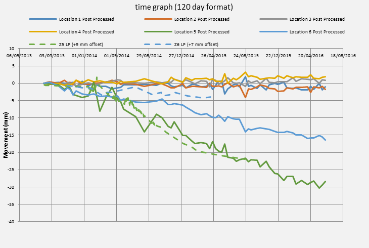
Figure 11: Comparison between InSAR processed data both inside and outside the ZOI at Bond Street vs manual levelling points.

5. Conclusions

Attitudes to monitoring are changing and most parties are becoming familiar with the need to analyse data in more appropriate ways to extract the value from it. In order to continue learning and improving the industry it is important that we take the following three conclusions from this paper into account for future projects:

1. Plotting movements in more detail (with a thinner pen, as per Figure 6 & Figure 7) does not provide greater assurance to stake holders. It is necessary to put things in to perspective and context, and to make sure that all the stake holders understand what is being shown. Sometimes a thicker pen will show trends better by accommodating possible noise, and might even show bigger scale patterns like an annual. For this we recommend:
2. Use a proper movement scale, if the expected movements are of certain scale uses that as a limit to present the results. Triggers can be shown on the plot to illustrate levels of risk.
3. When plotting several results taken over the same day (such as automatic monitoring every hour), use a median to present that data in that one day, skipping the more detail data unless it adds value to someone (such as compensation grouting). This will make the data coming from different sources more comparable and will take out of the equation the most abnormal values due to high or low temperatures or spikes.
4. When plotting the data it would make more sense to plot the entire history for that sensor (or group of sensors), that will help to spot abnormal behaviours, and will bring movements in to context assisting to understand the repeatability of that specific sensor.
5. New technologies at some point will become standard practice, and it should be in everyone’s interest to test them against the more traditional systems in order to understand them better and test their potential uses.
6. The absence of accepted industry standards for optical monitoring systems can lead to ambiguities and misconceptions in technical specifications. Using a specific instrument does not guarantee the precision, accuracy or repeatability quoted in the monitoring readings. We provide an indication on what is thought to be realistic in Table 3, but the monitoring contractor should always provide what is achievable with the different systems in the different areas taking in the various constraints. If possible he should provide simulations or justifications for them.

The client and designer should be the responsible for understanding what is necessary to be measured, how this should be made, and providing a suitable design for it (with considerations). The Contractor and Principal Contractor should be responsible for providing realistic estimations of what they can achieve and guaranteeing that the available ISOs or standards have been followed.

6. Acknowledgements

Thanks to Pietro Bologna (ARUP), Toni Laque (ERDA, Martin Beth (Soldata Group)) and Simon Nevard (Crossrail) for their assistance and comments to get this paper finished.

7. Bibliography

[1] Burland, J. B. (1995). Assessment of risk of damage to buildings due to tunnelling and excavations. Proceedings, 1st International Conference for Earthquakes and Geotechnical Engineering.

[2] Cording, E. J. (2005). Assessing movement and damage due to underground construction. Underground Construcion in Urban Environments. New York City: ASCE.

[3] Crossrail. (2010). Civil Engineering Design Standard, Part 8. Assesment of existing stuctures and mitigation design.

[4] Devriendt, M. (2005). Alternatives to the gaussian curve approximation – A comparison of empirical and analytical tunelling induced ground movement analyses in fine grained soils. Underground Construction.

[5] Dunnicliff, J. (1993). Geotechnical instrumentation for monitoring field performance. Wiley.

[6] Gonzalez Marti, J., Brzeski, J., & Sanchez Barruetabena, J. (2016). Realistic expectations while monitoring with netword robotic total stations systems in live rail environments. Crossrail Project: Infrastructure design and construction, Volume 3, pp. 369-392.

[7] Jones, L. D., & Jefferson, I. (2012). Chaper 5 – Expansive Soils. In ICE Manuals. 413-441: ICE Publishing.

[8] Lian, Z. (2015). Influence of ambient temperature on building monitoring in urban areas during the construction of tunnels for transportation. Universitat Politècnica de Catalunya. Departament d’Enginyeria Civil i Ambiental.

[9] Mair, R. J., Taylor, R. N., & Bracegirdle, A. (1993). Subsurface settlement profiles above tunnels in clays. Geotechnique, 315-320.

[10] Mair, R. J., Taylor, R. N., & Burland, J. B. (1996). Prediction of ground movements and assessment of risk of building damage due to bored tunnelling. International Conference of Geotechnical Aspects of on Underground Construction in Soft Ground, (pp. 713-718). London.

[11] Standing, J. R., Withers, A. D., & Nyren, R. J. (2001). Measuring techniques and their accuracy. Building response to tunnelling: case studies from construction of the Jubilee Line Extension, London, 273.