The use of InSAR (Interferometric Synthetic Aperture Radar) to complement control of construction and protect third party assets
Document
type: Case Study
Author:
Javier González Martí MSc MBA, Simon Nevard MSci ARSM, Jordi Sanchez MSc MSc GIS
Publication
Date: 19/09/2017
-
Read the full document
Introduction and Industry Context
InSAR (Interferometric Synthetic Aperture Radar) is a monitoring technique that compares the phase of two SAR measurements in order to determine the relative ground movement between the measurements.
InSAR was used to complement traditional ground movement monitoring techniques for the control of construction works and protect 3rd party assets on the Crossrail project.
SAR measurements use satellite-based radar. An antenna emits microwave electromagnetic radiation which is reflected by the Earth’s surface and returns to the receiver. Measuring the time taken for the radar energy to be returned and the change in frequency between the emitted and returned signal due to the Doppler Effect allows the position where the radar energy interacted with the ground to be calculated. Several signals are combined as the satellite travels through space, effectively increasing the aperture size to allow high resolution images to be produced [4].
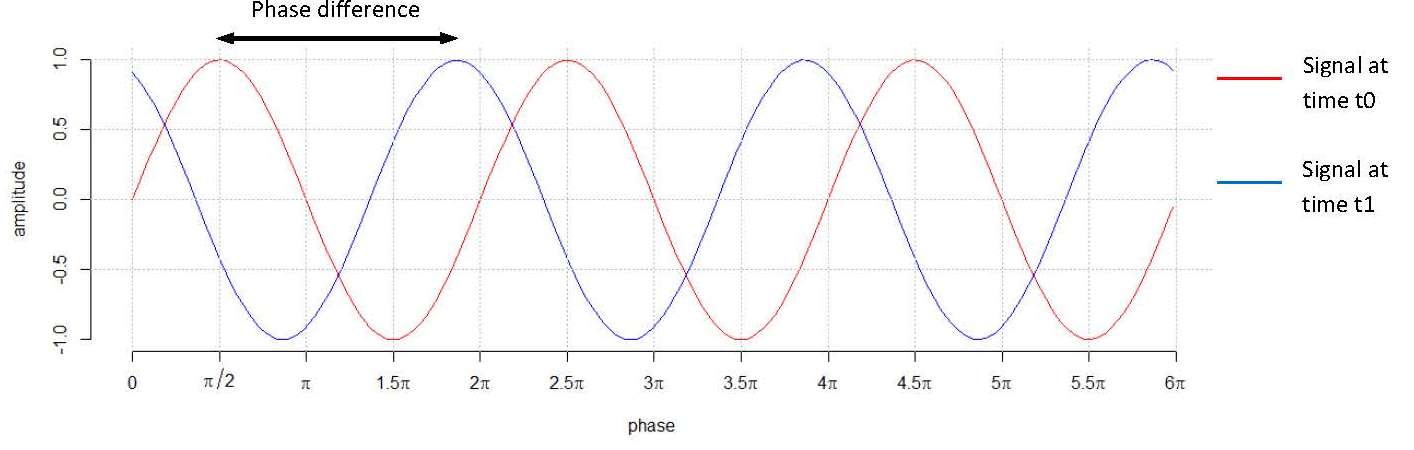
Each pixel in a SAR image consists of the amplitude and phase of the returned radar energy (see Figure 1). For a particular pixel, the difference in phase between two readings taken at different times can be calculated [3]. If the ground position has changed over time, the radar energy will take a different amount of time to return to the receiver for each reading and therefore have a different phase. Calculating the phase difference for all pixels in a pair of images allows an interferogram to be produced. Once corrections to remove noise have been applied, the remaining phase differences indicate relative ground movement between the two readings. Sources of noise include atmospheric effects and varying satellite orbits. InSAR relies on subsequent measurements being taken in the same spatial position, however, a satellite’s position may vary by several metres between each set of measurements. The variation will cause a shift in phase across the entire set of measurements which can be identified and removed (by measuring the perpendicular baseline between the satellite’s orbits) [2].
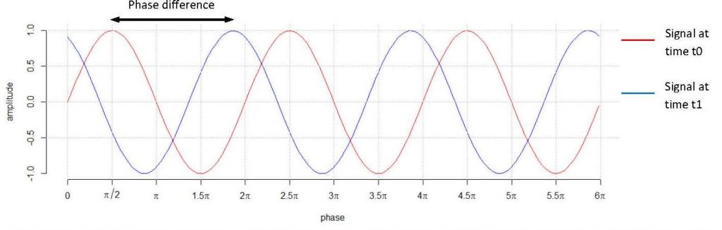
Figure 1 – Plot showing the relationship between phase and amplitude of a SAR signal at initial time, t0, and at a later time, t1, where the position of the Earth’s surface has changed.
On the Crossrail project, the satellite-based antennas emit X-band electromagnetic radiation (31mm wavelength). This limits the maximum observable movement of a pixel between two observations to 15mm. The minimum time between images was limited to 11 days due to satellite orbit times. These limitations mean InSAR is not a suitable method to monitor construction works where rapid, large ground movement greater than 15 mm between readings is expected and requires daily monitoring, however, InSAR is useful to monitor ground movements post-construction where the expected movement is small and monitoring is required less frequently. It is also useful to collect pre-construction baseline data in order to estimate ground and/or structure movement due to factors other than construction activity, such as seasonal temperature variations and seasonal variations of the phreatic conditions. For the Crossrail project it was envisaged that the data collected by InSAR would be able to provide enough robust data in order for other to assess the stability of ground and structures in the Crossrail zone of influence.
This paper presents several case studies and discusses how InSAR was used on the Crossrail project, limitations of the technique, potential cost savings against more traditional monitoring techniques, recommendations for future projects and a review of the use of InSAR data in various GIS software packages.
InSAR data used on the Crossrail project was collected via two TerraSAR-X satellites (made by Airbus Defence & Space) in constellation. Images were produced every 11 days starting on 03/08/2013.
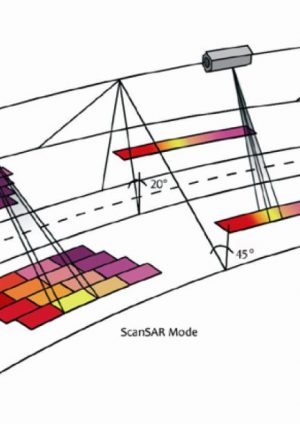
TerraSAR-X satellites have three standard modes of data collection: Spotlight, Stripmap and ScanSAR. In spotlight mode, radar is focused on a defined area as the satellite moves. This limits the image size but provides high resolution data. For TerraSAR-X, spotlight mode provides 10 km x 10 km images with 1 m resolution (a pixel size of 1 m x 1 m). Data for an indivual pixel is the result of the constructuve and destructive summation of signals backscattered over that area.
In Stripmap mode, radar is pulsed continuously as the satellitle moves, producing data in a continuous strip. This provides images with a lower resolution than spotlight mode but over a larger area. TerraSAR-X images in stripmap mode are 30 km x 50 km and have 3 m resolution. In ScanSAR mode the antenna moves to image several continuous strips as the satellite moves.
ScanSAR mode enables data to be collect over large areas (100 km x 150 km) at the cost of lower resolution (16 m to 18 m). For all data collection modes the accuracy of the vertical distance measurements are the same because this depends on the wavelength of the emitted signal. The modes of data collection are summarised in Figure 2. On the Crossrail project, data was collected in Stripmap mode.
The Crossrail InSAR data was processed with a technique known as Persistent Scatterer Interferometry (PSI). This technique identifies points that reliably backscatter the radar signal in each set of measurements. These points are known as persistent scatterers. Objects that are subject to frequent movement (such as vegetation) and objects with a low backscatter coefficient (focusing of backscattered signals away from the radar source) , smooth surfaces such as lakes, are poor persistent scatterers and PSI InSAR coverage is therefore sparse in areas of vegetation and still water but generally of high density in the vicinity of buildings and pavements which have high backscatter coefficients (focusing of backscattered signals towards the radar source).

Figure 2 – Methods of data acquisition, from TerraSAR-X Image Product Guide (Airbus Defence and Space)
Case Study 1 – Whitechapel
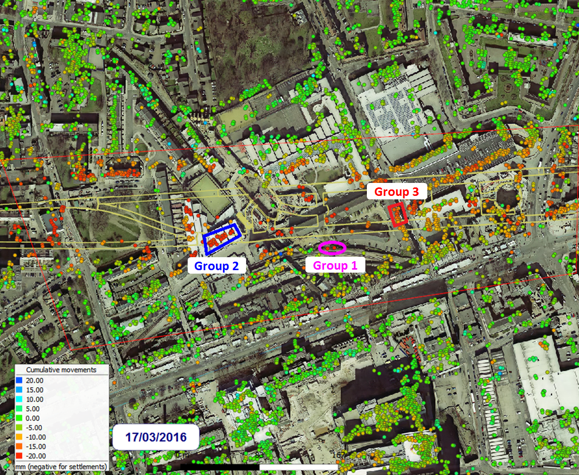
InSAR coverage for Whitechapel is summarised in Figure 3.

Figure 3 – Plan showing InSAR coverage at Whitechapel.
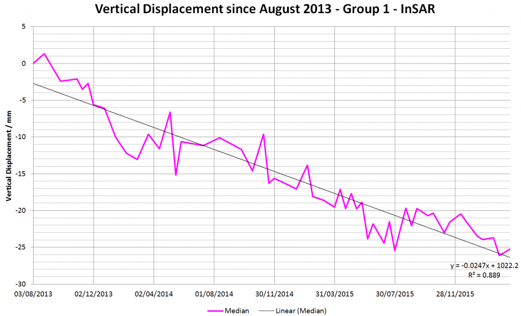
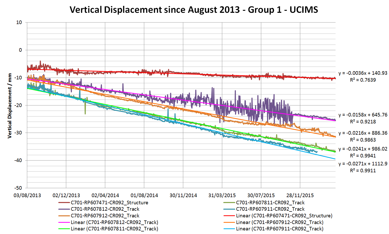
Figure 4 – Group 1 InSAR results

Figure 5 – Group 1 automated prism results with linear regression trend lines
Conventional automated monitoring of prisms on London Underground (LU) and London Overground (LO) assets at Whitechapel was undertaken between March 2012 and May 2016. Conventional manual levelling of points installed on buildings and streets in the vicinity of LU and LO assets at Whitechapel commenced in May 2012 and is ongoing at the time of writing this case study. This monitoring data is stored in the Crossrail online database UCIMS (Underground Construction Information Management System).
Three months after completion of Crossrail works at Whitechapel that had the potential to cause ground settlement, UCIMS data generally suggested that, as expected, the rate of settlement across the site had reduced to less than 2 mm per year, with the exception of a small area in the vicinity of the LU Station (see Figure 3, Group 1). UCIMS track monitoring data (see Figure 5) indicated settlement in this small area had been continuing at a steady rate of approximately 8 mm per year since monitoring commenced in March 2012. This trend was not observed in structural monitoring data. Crossrail works that had the potential to cause settlement in the vicinity of Group 1 had not commenced in March 2012 which suggests the settlement was caused by other sources such as the condition of track ballast or local geology.
Following decommissioning of the prism monitoring system, InSAR was used to monitor LU and LO assets at Whitechapel. Only two persistent scatterers were available in the vicinity of the anomalous settlement area. While this is a small sample size, the two persistent scatterers very closely matched the UCIMS track monitoring data (see Figure 4 and Figure 5), indicating a fairly continuous settlement rate of approximately 9 mm per year since August 2013.
InSAR has been a useful tool to complement the existing monitoring in this area and is more cost effective than maintaining the automated prism monitoring system, or undertaking this monitoring manually. Provision of InSAR data for the entire Crossrail central tunnelled section, including purchasing of images, data processing and management and provision of a quarterly report costs in the tens of thousands of pounds (depending on number of pictures per period and other factors), while maintaining automated prism monitoring and manual monitoring across the same extent would be in region of hundreds of thousands of pounds. Of course the information obtained by these three different systems is in a way different, and they should complement each other depending on the specific constraints at a site.
However, as there are only two persistent scatterers available in Group 1 at the time of writing, there is a risk future images may cease to have sufficient coverage.
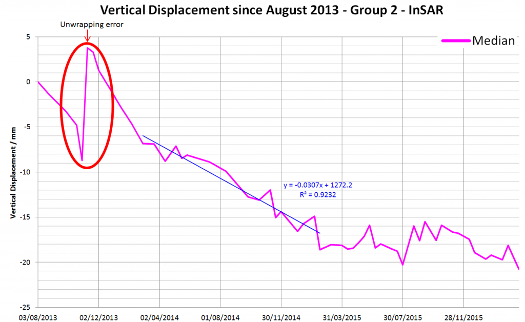
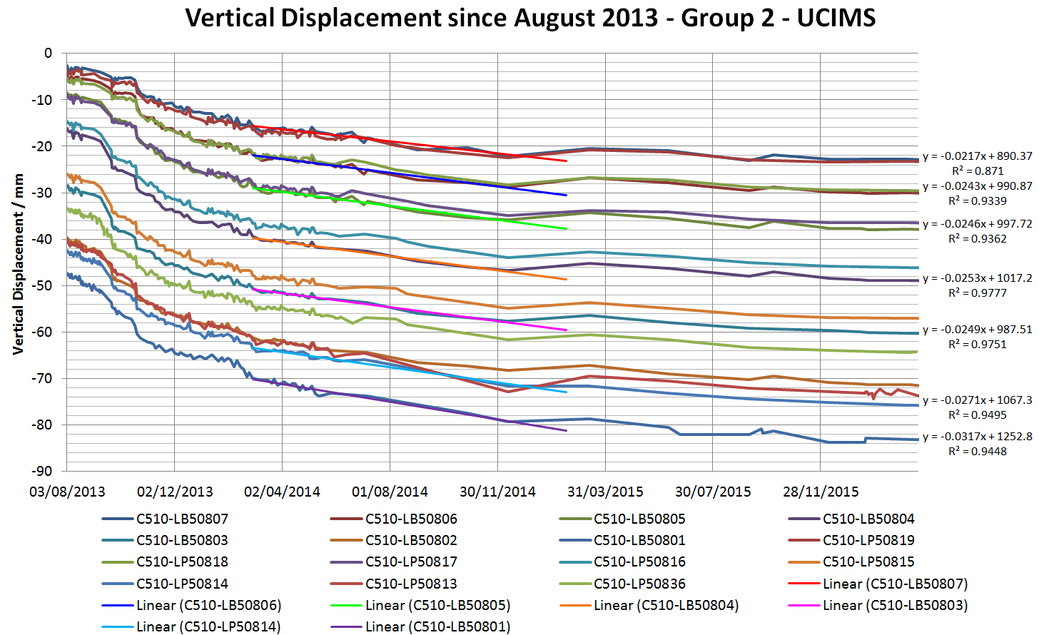
Figure 6 – Group 2 InSAR results with linear regression trend line between 28/02/2014 and 15/02/2015
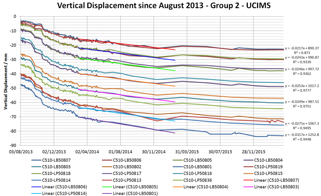
Figure 7 – Group 2 manual levelling results with linear regression trend lines between 28/02/2014 and 15/02/2015
Comparison of InSAR and manual levelling results for group 2 on the roof of the Whitechapel Sport Centre indicate an error with phase unwrapping in late 2013 (see Figure 6). Raw phase values are measured on a repeating scale between 0 and 2π radians (see Figure 1). When data is processed, a multiple of 2π is added to the raw phase value in a process known as unwrapping [4]. Adding an incorrect multiple of 2π to the measured phase value will result in an inaccurate estimate of ground movement.
Unwrapping errors are likely to occur in areas where there are high phase gradients from pixel to pixel, for example, in areas of rapid ground movement. Where a phase difference greater than π is measured between two adjacent pixels, the correct multiple of 2π to add to the raw phase value cannot be determined. InSAR data used on the Crossrail project uses X-band electromagnetic radiation with a wavelength of 31mm. Therefore, differences of more than 15mm between adjacent pixels (in space or time) will result in unwrapping errors. As images were only captured every 11 days, InSAR was not a useful tool for monitoring ground movements during construction, as movements of greater than 15mm were likely to occur between images in some cases.
With the exception of the phase unwrapping error, the settlement rate measured via InSAR is similar to the rate measured by manual levelling, although the rates do not exactly match (see Figure 6 and Figure 7). The difference is likely to be due to InSAR producing absolute measurements whereas traditional monitoring techniques are referenced to local datums (this will be discussed further in the review of Group 3 data below). The InSAR persistent scatterers are located in slightly different positions to traditional monitoring points which may account for further differences in the data. Offsets can be manually applied to InSAR data to correct for phase unwrapping errors and offsets have been applied in some areas. However, several instances of unwrapping errors remain in the Crossrail data as the errors need to be identified manually and offsets applied manually; a process that takes significant amounts of time. Calculating absolute settlement values using InSAR data may not be possible, however, InSAR data is still useful to calculate relative settlement rates providing care is taken when selecting the time period for the calculation.
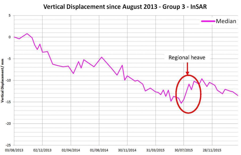
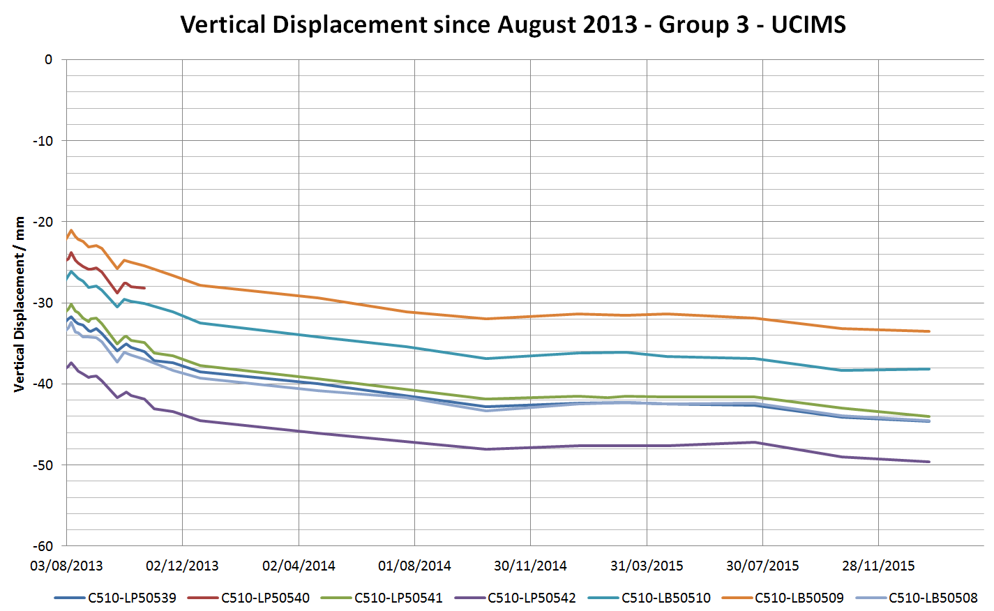
Figure 8 – Group 3 InSAR results
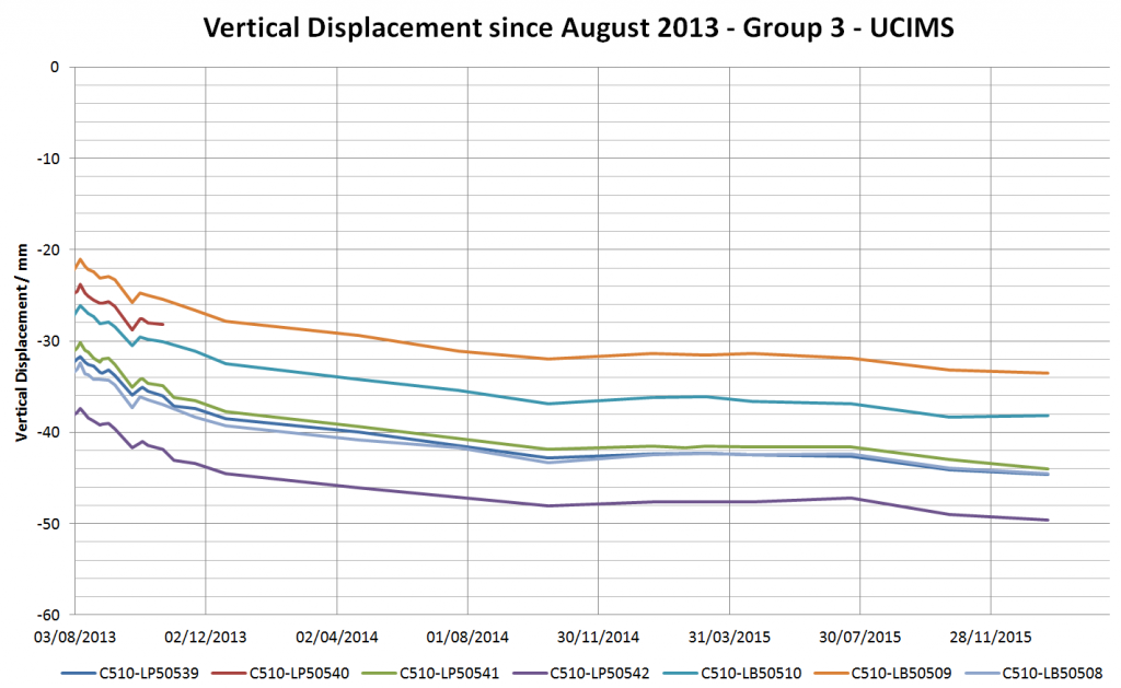
Figure 9 – Group 3 UCIMS results
Results for Group 3 (Figure 8), on the top of the Kempton Court buildings, show a potential advantage of using InSAR for post-construction monitoring rather than conventional surveying techniques. On the Crossrail project, the purpose of post-construction monitoring was to demonstrate that settlement rates within the Crossrail zone of influence had reduced to less than 2 mm per year. Low settlement rates were expected once construction of Crossrail assets was completed so low frequency manual monitoring (one survey every few months) was deemed as sufficient to monitor post-construction settlement rates. InSAR provides data every 11 days, a much higher frequency than the chosen manual monitoring frequency, and at a lower cost than manual monitoring for such a wide area.
As InSAR is not affected by regional movements, whereas traditional monitoring methods are referenced to a local datum, the real behaviour of the entire monitored area was measured via InSAR (Figure 8). This movement was not measured by the manual monitoring in the area, which shows a more stable behaviour (Figure 9), because both the monitoring points and the datum that they are referenced to were subject to the same regional (non-Crossrail construction related) movements.

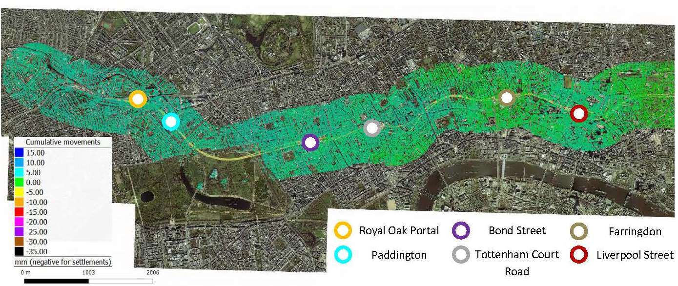
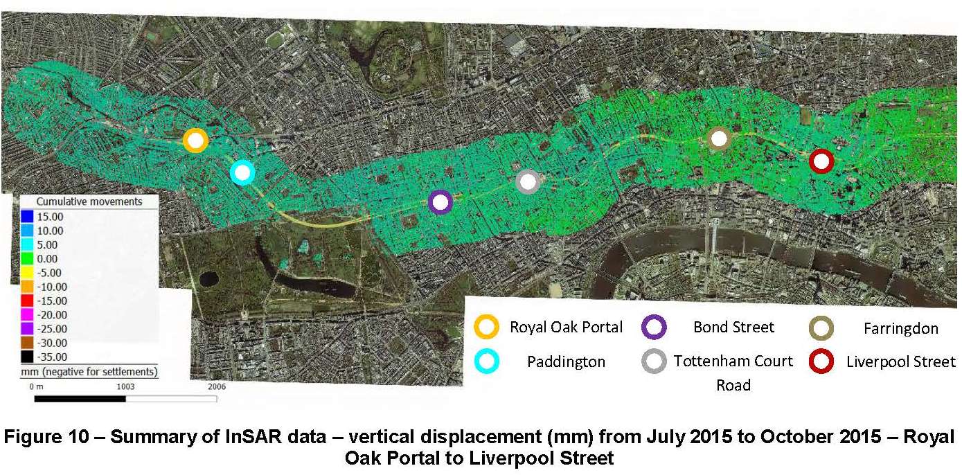
Figure 10 – Summary of InSAR data – vertical displacement (mm) from July 2015 to October 2015 – Royal Oak Portal to Liverpool Street
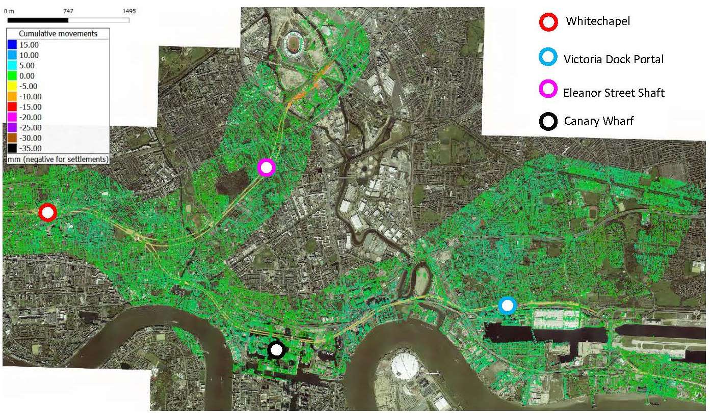
Figure 11 – Summary of InSAR data – vertical displacement (mm) from July 2015 to October 2015 – Whitechapel to Victoria Dock Portal
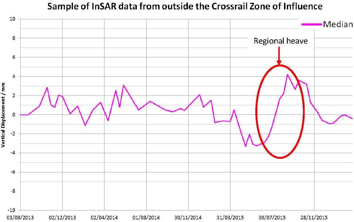
Figure 10 and Figure 11 show differential movement between July 2015 and October 2015 observed in InSAR data. Between approximately July 2015 and October 2015, InSAR has measured a regional heave trend followed by gradual settlement until December 2015 which has affected areas from Paddington to Canary Wharf. The trend has been observed from areas outside of the Crossrail zone of influence (see example in Figure 12), with no other known construction influences present which could cause this movement. The availability of InSAR data outside the Crossrail zone of influence allowed for the cause of this anomaly to be attributed to (undetermined) factors unrelated to Crossrail.
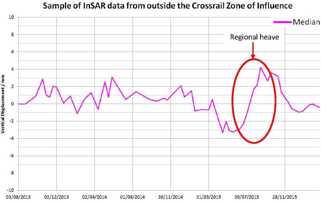
Figure 12 – InSAR data from outside the Crossrail Zone of Influence showing regional movements
Case Study 2 – Farringdon
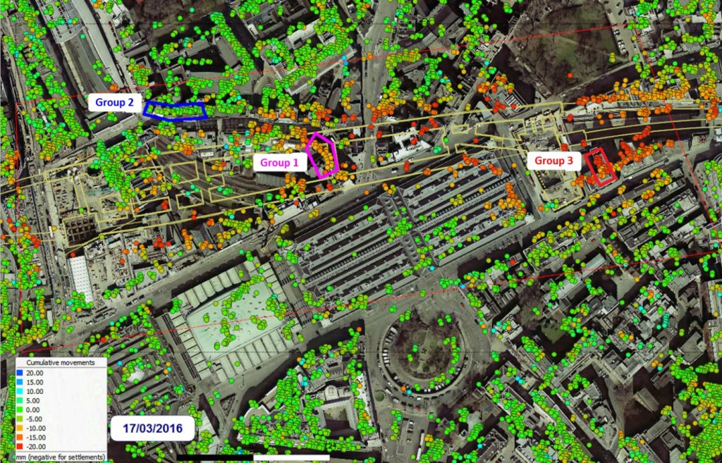
Figure 13 – Plan showing InSAR coverage at Farringdon Station
InSAR coverage at Farringdon Crossrail Station is generally dense in the vicinity of buildings and sparse in areas of vegetation. Groups 1 and 3 are buildings within the Crossrail zone of influence. Group 2 is slightly outside the zone of influence of the Crossrail works.
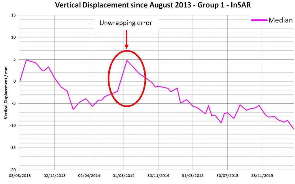 Figure 14 – Group 1 InSAR results
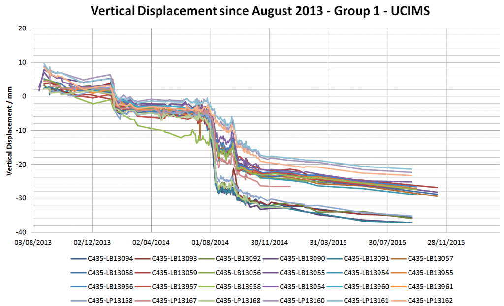
Figure 15 – Group 1 UCIMS results
Traditional monitoring data in Figure 15 from UCIMS for group 1 indicates rapid settlement in August 2014. This coincides with tunnel enlargement works using sprayed concrete lining (SCL) techniques and was therefore anticipated. The data suggests the SCL works caused between approximately 10mm and 20mm settlement. InSAR data (see Figure 14) shows that settlement of greater than 10mm between two readings produces unwrapping errors. This is a limitation of InSAR and can only be corrected by manually applying offsets (e.g. to match nearby manual monitoring points) to the processed InSAR data.
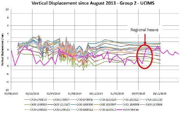
Figure 16 – Group 2 InSAR results vs UCIMS results
Group 2 InSAR data has a good correlation with nearby manual levelling points. The regional heave trend is present in the InSAR data although is not observed in the UCIMS data, likely due to benchmarks for the manual monitoring also moving due to the regional heave.
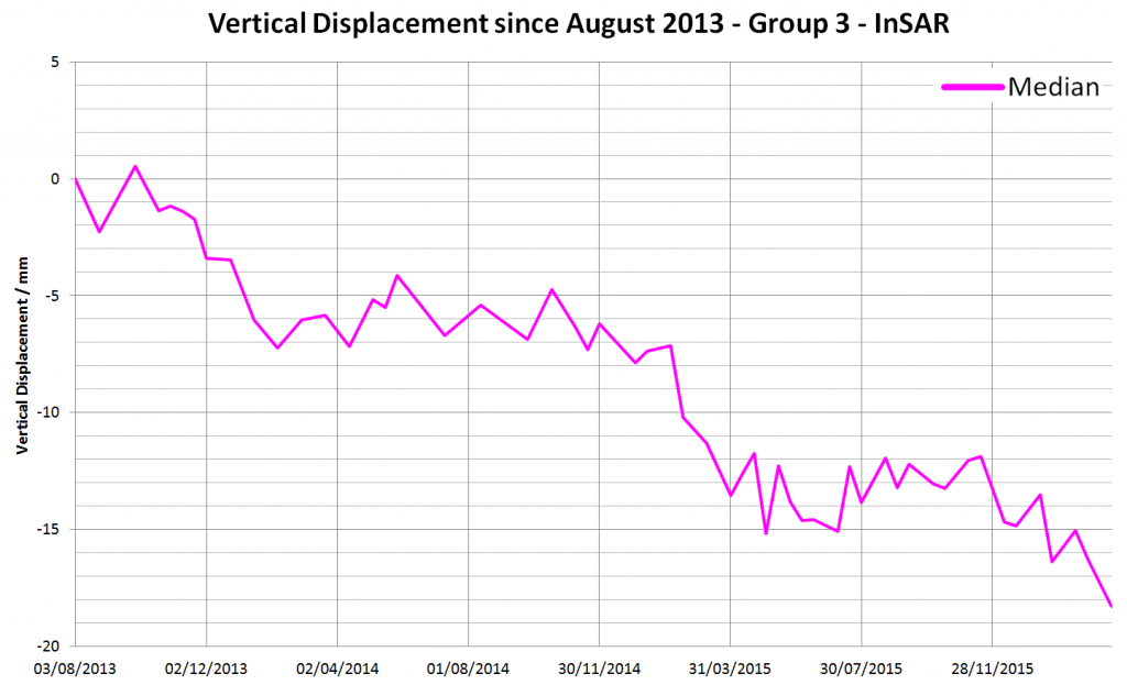
Figure 17 – Group 3 InSAR results
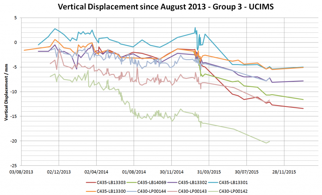
Figure 18 – Group 3 UCIMS results
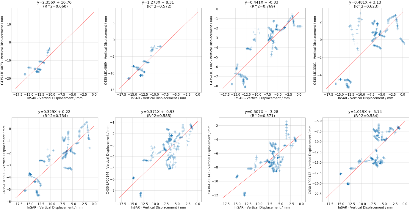
Certain manual levelling points in group 3, such as C430-LB133302, show a good correlation with group 3 InSAR data. Other manual levelling points in the group do not correlate as well (see residuals in Figure 19). This may be because levelling points are fixed to the building façade at ground level or to the pavement (and are relative to the main benchmarks), whereas InSAR persistent scatterers are generally on the roof of buildings (and are absolute).
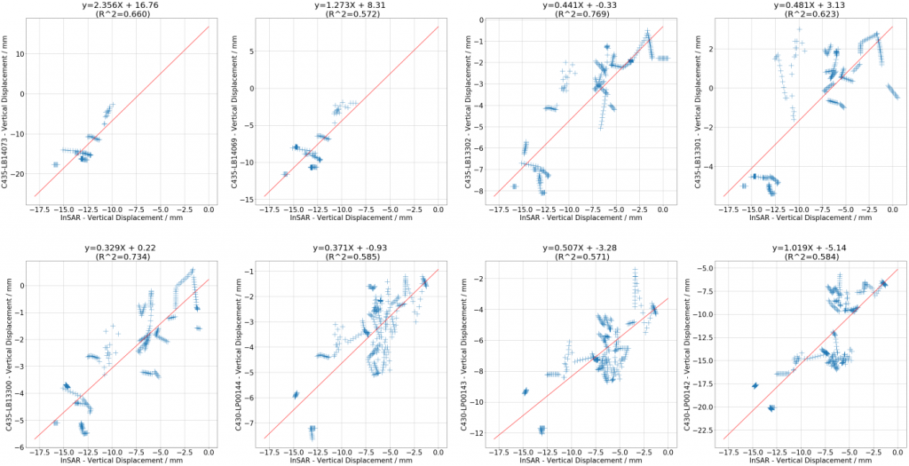
Figure 19 – Linear regression trend lines comparing the correlation between InSAR data and manual monitoring points for Group 3 (with limited linear interpolation for missing values in order to align timestamps)
Case Study 3 – Unwrapping error during TBM Passage
Unwrapping errors when processing InSAR images can conceal ground movement episodes requiring posrt analysis and mitigation to reflect the reality. During the TBM passages between Whitechapel and Liverpool Street stations some pixels identified the settlement produced by the excavation in both occasions while there were areas that captured settlement over a period of time as heave.
the InSAR settlement data from the TBM passages in December 2014 (1st TBM passage) and February 2015 (2nd TBM passage); the boring machines drives were spaced approximately two months apart, allowing a sufficient period for detection of the ground movement . As shown on Figure 20, the two areas studied are approximately 90m apart and at the same position above the alignment. Group 1 shows settlement trends consistent with the TBM passages (Figure 22), while Group 2 does not feature the expected trends.
Figure 20 – Areas displaying different reaction to the TBM passages
The rapid nature of the ground reaction to the TBM passages and the amount of settlement produced by the works (around 10mm in that area) results in an unwrapping error that still captures the movement produced but does not identify the real direction of movement.
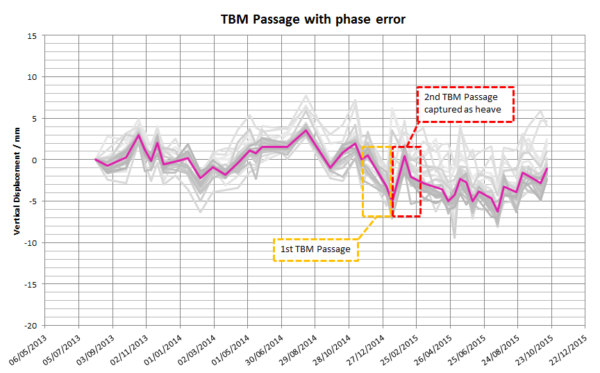
Figure 21 – InSAR data not reflecting one of the TBM passages
Figure 21 shows how the second TBM passage apparently compensates the movement from the first one.
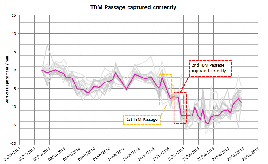
Figure 22 – InSAR data corrected to properly represent TBM passages
Figure 22 displays the correct interpretation made by the contractor’s software with the TBM drives’ settlement represented for Group 1. The solution to these kinds of system glitches is to apply an offset on the InSAR data in the relevant area from a given point in time based on other readings available (such as manual monitoring or nearby more reliable InSAR data). As previously stated, InSAR monitoring in this instance is not adequate to monitor active works that can produce big settlements (beyond 15 mm) in a short period of time, but without a doubt is complementary.
During the early stages of the InSAR contract, a comprehensive review was done of the main areas of Crossrail’s works in order to mitigate the unwrapping errors effect found along the alignment. This effort translated into the retrospective review of the data from 2013.
Due to the extent of the InSAR coverage, the entire dataset has not been subject to a detailed review. Further offset corrections could therefore be made.
Software provided
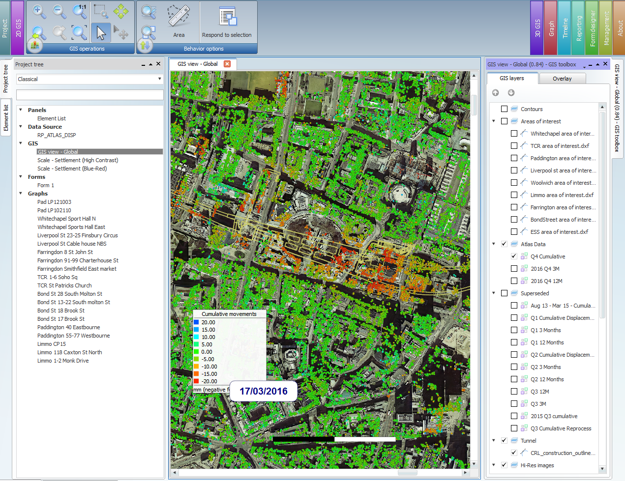
The software supplied with the data, Geoscope 7, falls in the range of the GIS visualizers; it presents geospatial data in different layers such as map tiles, vector maps and points but lacks geospatial calculation and layer interaction features amongst other typical GIS functions.
InSAR data is provided quarterly under this contract and is added to the software’s layer library, the latest data is shown in the layer tree separated from the previous superseded one. Additional aerial photography and Google Maps layers are also included as background. The Crossrail project layout is included as a vector layer (see right hand “GIS Layers” on figure 23).
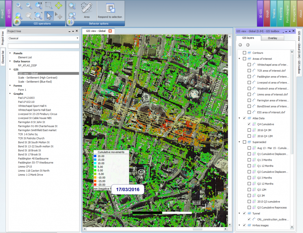
Figure 23 – Geoscope 7 InSAR data visualizer
Once the software has populated the view, which can take several minutes due to the large amount of data, detailed plots can be requested by selecting clusters of points and defining the relevant coordinate (Northings, Eastings and level (Z)). Time plots can be generated, saved, exported, etc. using the different features available.
The package is able to present time plots and export data reasonably quickly. The key in the processing speed is the fact that the readings are installed locally, as opposed to other web-based visualizers that require real time online database queries.
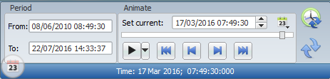
Figure 24 – Geoscope 7 Timeline animation controls
Geoscope 7 is capable of displaying settlement data throughout time using the “Timeline” function, this tool is similar to the one used in ArcGIS (See Figure 25) and other Open Source software such as QGIS. At the time of the writing this function is still in development as it requires improvement. These kinds of animations are helpful when briefing stakeholders about the behaviour of the ground surrounding the project over time.
Use of third party software on InSAR data

Figure 25 – InSAR data displayed through ArcGIS software
InSAR data is also provided in the form of comma separated value (CSV) files which can be used to feed GIS software and/or Geodatabases. This enables more options of data usage and interaction. ArcGIS has been used to evaluate the potential of quick geospatial queries and report elaboration. Simultaneously, the C704 IT Developers’ team is also working on the integration of InSAR data in the next iteration of the UCIMS platform, which will feature geospatial query capabilities. AGS file import/export will potentially be a feature of the software although this is in development at the time of writing.
The formatting of the CSV files used with ArcGIS needed reworking before they could be uploaded in an ESRI geodatabase file. Each file had to be split into many and each reading had to be linked with a unique timestamp; this happens as a result of the CSV file structure which was not designed to be used in such way.
When using a fully featured GIS software, InSAR data can be complemented with additional vector or raster layers as long as they are in the same coordinate system. Building layers can be added and queried in conjunction with InSAR data based on the building’s metadata; such as address, type of building, etc. Other assets such as stations or retaining walls which are usually tagged or labelled and can be linked to settlement values. With a simple query the data regarding any relevant structure can be located and linked to it, relating movement trends with any other metadata available.
Established GIS platforms have been developing the use of time-enabled layers for several years. Once the InSAR data is loaded as a time-enabled layer it can be combined with other similar layers to create animations such as SCL advances, compensation grouting episodes, etc. (see Figure 25). The functionality of this feature in other software is better than Geoscope 7 at the time of this writing, although the maximum advantage is gained by the amount of layer interaction rather than animation software by itself.
Figure 26 – Cumulative InSAR data and SCL advances at Bond Street up to 27/05/2014 and compensation grouting injections (volumes injected only on the 27/05/2014)
Lessons Learned and Recommendations for Future Projects
Evidence from the case studies presented suggests that the main limitations of InSAR are the frequency of images and wavelength of electromagnetic radiation emitted.
Image frequency depends on the number of satellites in constellation. There were two TerraSAR-X satellites in constellation that were used on the Crossrail project, allowing images to be produced every 11 days. This limitation means InSAR was not suitable to detect rapid ground movements, such as those produced during the construction of Crossrail tunnels and stations. InSAR was useful to monitor post-construction ground movements, where the settlement rate is lower and large settlement rates are not expected. Calculating absolute settlement values using InSAR data may not be possible, however, InSAR data is still useful to calculate relative settlement rates providing care is taken when selecting the time period for the calculation. Historical InSAR images allowed for non-Crossrail related ground movements to be assessed before monitoring via more traditional techniques had commenced. Future SAR satellite missions are planned which may allow for increased image frequency [1] [6].
TerraSAR-X emits X-band radiation with a wavelength of 31mm. This limits the maximum observable movement between adjacent pixels (in time or space) to 15mm. Movements greater than this will cause unwrapping errors. The case studies suggest that in practice, unwrapping errors may occur with movements of greater than 10 mm between measurements. This limitation also means InSAR is not a suitable tool to monitor rapid ground movements during the construction phase of a project.
The purchase and processing of InSAR data is very cheap compared to more traditional monitoring techniques such as geodetic prism monitoring via automated total stations or manual levelling. On the Crossrail project, the procurement and data management of InSAR data was approximately an order of magnitude cheaper than maintenance and data management of automated prism monitoring.
InSAR data also has the advantage of covering a very large area in a single image. The Crossrail project used satellites operating in StripMap mode, which produces an image size of 50km x 30km with a pixel size of 3m. Monitoring a similarly large area via more conventional monitoring techniques would not be practical and would be extremely costly. On the Crossrail project, monitoring of such a large area enabled a global heave trend to be identified that was caused by sources not related to the project.
InSAR is not recommended for use in rural areas as the unstable nature of vegetation and the smooth nature of water surfaces do not produce consistent backscattering towards the satellite [3]. Availability of persistent scatterers in cities is usually good although it is not guaranteed in all locations.
However, InSAR monitoring is recommended for use on future projects in urban areas to monitor both pre-construction and post-construction ground movement trends. It is not recommended for monitoring during construction as a unique source of information but can usefully complement more traditional monitoring systems with higher monitoring frequencies. Furthermore InSAR will provide data that will not be affected by local movements, as a potential benchmark could, therefore providing a measure of the true ground movements as a result of both local construction works and regional and global geological phenomena.
-
Authors


